Co-Authors: Alexandra Ebert & Daniel Soukup
In the previous part of this series, we have discussed two risks entailed in the rise of digitalization and artificial intelligence: the violation of the privacy and fairness of individuals. We have also outlined our approach to mitigate privacy and fairness risks with bias-corrected synthetic data: this allows for privacy-preserving data sharing and also aids the fair treatment of customers (data subjects) in downstream analysis and machine-learning tasks. (By the way, if you would like to experiment with fair synthetic data yourself, you can download the datasets we created at the bottom of the page.)
If you would like to dig deeper into algorithmic fairness and the potential risks in machine learning systems, we can highly recommend The Ethical Algorithm book by M. Kearns and A. Roth. For a more technical viewpoint, check out fairmlbook.org to find lecture notes, videos, and other great resources.
In this blog post, we take a deeper dive into our approach to de-bias synthetic data. For now, we focus on statistical parity as a fairness measure and show in detail the effects of our approach in two settings:
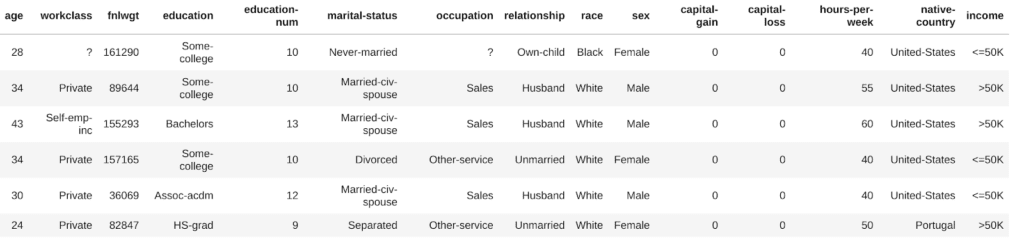
- the Adult US census data set, which is an extract of the 1994 US Census database, and
- the Compas recidivism data set that was the focus of ProPublica’s high profile machine bias study.
Read the other parts of the series:
- Part 1 - Why Bias in AI is a Problem & Why Business Leaders Should Care
- Part 2 - 10 Reasons For Bias In AI And What To Do About It
- Part 3 - We Want Fair AI Algorithms – But How To Define Fairness?
- Part 4 - Tackling AI Bias At Its Source – With Fair Synthetic Data
Statistical Parity as a Measure of Fairness
Let’s start with a quick reminder: a data set or algorithm being unfair usually refers to some kind of imbalance. A rather intuitive measure for such an imbalance is the so-called statistical or demographic parity. In mathematical terms, we can describe it as follows: consider a population that can be split into groups by a sensitive attribute S, such as gender, skin color, age or any other property. Then consider another target attribute T that contains sensitive information on the population such as income, whether or not people spent time in prison or credit history.
In the Adult data set, we select the sensitive attribute (S) gender, either “female” or “male”, and the target attribute (T) income, which is either “>50k” or “<=50k”.
In this example, statistical parity is satisfied when the number of females that earn more than 50K divided by the total count of females equals the number of males earning more than 50K divided by the total number of males:

In other words, the probability that a randomly chosen male is a high earner should be the same as the probability of a random female being a high earner. Also, note that when these two fractions are equal for the high-income segment (“>50K”) then this automatically holds true for the low-income segment (“<=50K”) as well.
In the real world, unfortunately, the equality above does not hold true. A simple visualization of the data set reveals a strong imbalance between females and males (Fig 2).
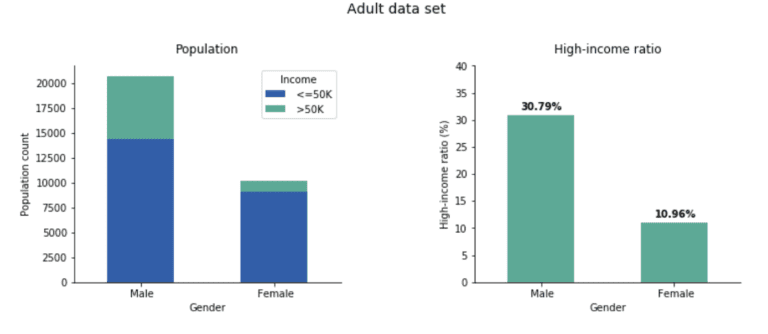
Only 10.96% of women are in the high-income range while among men, the fraction is 30.79%, almost three times higher. In the remainder of the blog post, we show how to create a fair, synthetic version of the Adult data set that removes the income gap between these two gender groups.
Though being intuitive, parity has limitations especially in the context of fair algorithmic decision making. We are aware of these shortcomings, some of which we mentioned in our fairness definitions post already, and we will discuss alternative fairness measures at the end of this blog post.
Generating a Fair Dataset
One of the first ideas to try when creating a fair data set for machine learning is to drop the sensitive column. In the presented case that’s the “sex” attribute. At first sight, this sounds like a good and easy-to-implement solution but, unfortunately, it can actually cause more harm than good. On one hand, what makes this approach fail can be so-called proxy or hidden proxy columns. Imagine we know which neighborhood a person lives in, the brand and model of the person’s mobile phone, the car this person drives, where this person buys her/his clothes, etc. Given some of the above information, we humans can make a pretty educated guess on this person’s sex, skin color, and other attributes. And since algorithms are better in analyzing patterns like this, they will definitely detect these correlations and exploit them, leading again to unfair predictions and decisions. We could actually go one step further and say that leaving the “sex” column in the data set is better for fairness because it offers a clear handle to enforce fairness constraints such as statistical parity. To give another example from criminal justice, women on average are less likely to commit future violent crimes than men with similar criminal records. So, a gender-neutral assessment can overestimate a woman’s recidivism risk.
Our synthetic data platform's community version is free to use and leverages deep neural networks to produce synthetic data. In order to generate fair synthetic data, we add a fairness constraint to the model parameter optimization during training. Sticking with the Adult data set, we penalize the violation of statistical parity within every mini-batch by increasing the training loss by a number that is proportional to the difference between the fraction of women and the fraction of men in the high-income segment. A very similar approach for training fair classifiers is described in a paper by P. Manisha and S. Gujar and an implementation can be found at Y. Shavit’s github repo.
In more general terms, adding the fairness constraint expands the objective of our software from generating accurate and private synthetic data to generating accurate, private, and fair synthetic data.
Private and Fair Synthetic Data
After feeding the Adult data set to our software and training it with the additional parity fairness constraint in place, we generate a synthetic fair version of the Adult data set. Once we evaluate the income distribution, we see a major change: the income gap almost disappeared (Fig 3).
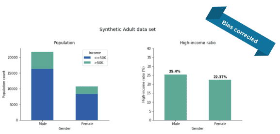
Actually, we repeated the whole process 50 times and the plotted numbers are the average ratios over these independent runs. The income-ratios slightly varied across the 50 experiments but this variance (rooted in the stochastic nature of our training and generation process) was quite small: 1.2% and 1.3% for the Male and Female ratios, respectively. As apparent from the plots, the synthesis corrected the income gap: 25% of the synthetic males are high earners (instead of the real 30%) and 22% of the synthetic females are high earners (while the original value was 11% only).
With regards to parity, it is common to compare not just the difference but the fraction of high-income male ratio to high-income female ratio (that is, we divide the two sides of the above equation). This fraction is called the disparate impact and it is an industry-standard to ask for at least 0.8, the so-called four-fifth rule. In the original data set, this fraction is roughly 10/30 = 0.33, a quite severe disparate impact violation but the bias-corrected synthetic data is at 22/25 = 0.88, well over the threshold.
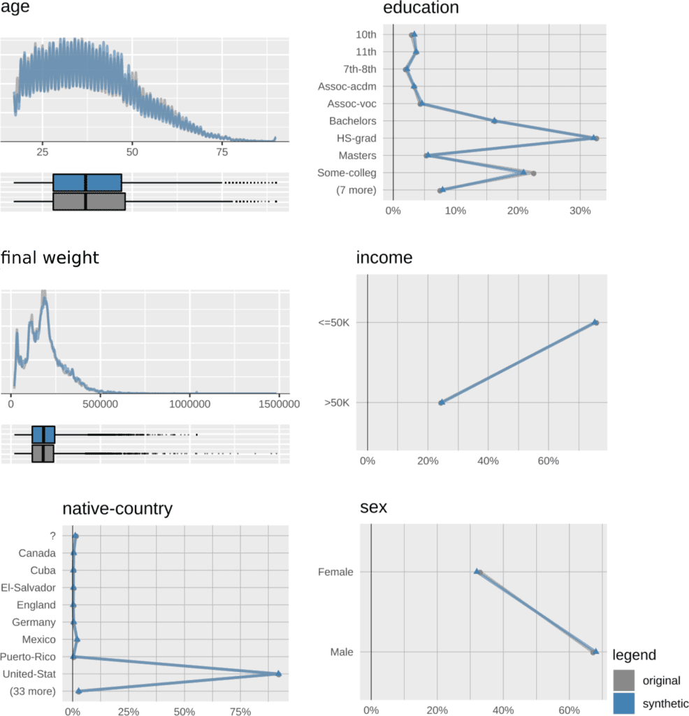
The additional parity constraint during model training does not diminish the quality and accuracy of the synthetic data. Univariate distributions of the synthetic-data attributes almost perfectly match their original counterparts (in Figure 4, we show only a selection). Please note that, while parity is modified to a large degree, both the population-wide male-to-female ratio, as well as the high-earner-to-low-earner ratios, are preserved.
Also the bivariate correlations of the synthetic data, on first sight, seem to be in excellent agreement with the original data (Figure 5).

A closer look, however, reveals some detailed changes due to the inner workings of the fairness constraint. Given the statistical parity definition, “income” must not depend on “sex”, which means these two attributes should not be correlated.
While in the original data, there is a clear “sex”-”income” correlation (red circle in the left plot in Figure 5) this dependency is almost reduced to noise level in the fair, synthetic data (red circle in the right plot in Figure 5). Apart from the “sex”-”income” pair, no other correlation seems to be altered by applying the fairness constraint, at least not strong enough to show a visible effect on the correlation plot.
But what about proxy attributes, columns in the data set that are correlated with “sex” and “income”? Can they introduce unfairness through a backdoor, as they are not explicitly mentioned in the parity constraint? Recall that the “parity equation” (see Equation 1) contains the attributes “sex” and “income” only.
To visualize the effect of the parity constraint on proxy attributes, we add an artificial feature to the Adult data set named “proxy”. We generated this column so that it is strongly correlated with the attribute “sex”. For females, “proxy” equals to 1 in 90% of all cases and equals to 0 for the remaining 10%. For males, the percentages are swapped. Looking at this new data set, we see, first, the strong correlation between “sex” and “proxy” (the black arrow on the left-hand side plot of Figure 6). Second, as these two attributes are strongly linked, also their correlation to “income” is comparable (the red arrow on the left-hand side plot of Figure 6). Now, when we run our synthetic data solution with the fairness constraint in place on “sex” only, we find that in the fair synthetic data both correlations “sex”-”income” and “proxy”-”income” are almost reduced to noise level (the red arrow on the right-hand side plot of Figure 6). The latter finding shows that the parity constraint works as intended and accounts for (hidden) proxy attributes.

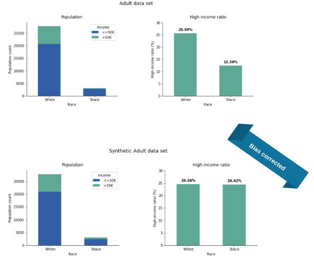
In the Adult data set, gender is not the only sensitive attribute: if we train our synthetic engine with “race” as a sensitive attribute, we get similarly impressive corrections (for this task, we used a simplified version of the data set filtering for Black/White subjects). In the original data, there are twice as many high earners in the White population than in the African American, but the ratios are almost exactly equal in our adjusted synthetic data (Figure 7).
In summary, the introduction of (parity) fairness to our software solution shows very promising results. The quality and accuracy of the synthetic data remain high, the privacy of data subjects is protected, and parity-fairness is guaranteed. All these properties make private and fair synthetic data readily available for further application.
Mitigating Bias on More Than One Feature
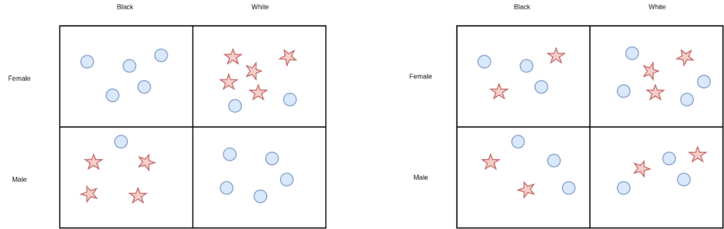
It is also a possibility to turn on the fairness loss on multiple sensitive attributes at the same time which we did for race and gender. In this case, one must be careful what ratios to optimize: if we were to simply put fairness losses independently on race and gender then the algorithm might fall into the mistake of “fairness gerrymandering”. That is, the new data set would look fair with respect to both gender and race individually, but we would see high imbalances when restricted to gender and race simultaneously (Figure 8).
Taking this into account, our solution gives synthetic data with significantly balanced high-income ratios across the four groups given by race and gender (Figure 9).
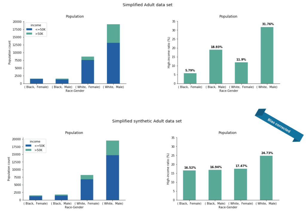
It is apparent that we did not achieve complete parity but this difference can be further lowered by giving higher weight to the fairness loss against the accuracy loss.
Fair Synthetic Data in Downstream Machine Learning Tasks
In the previous post, we introduced a scenario in which Got Big Data Company generates a fair synthetic dataset. This data set is handed to an external vendor, SmartUP AI, to develop new predictive models. As the data set is fair and synthetic, SmartUP AI does not need to take specific privacy measures nor does it need to apply any bias correction so they can work with standard, out-of-the-box models.
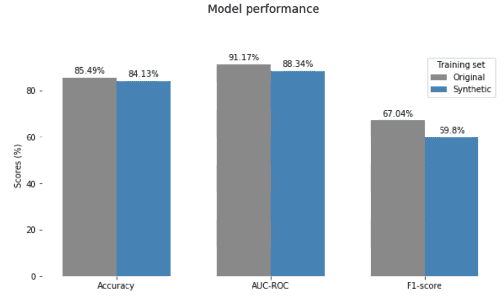
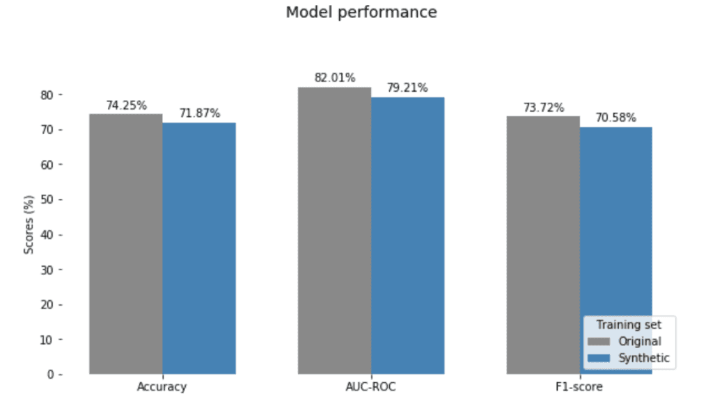
We demonstrate this with the Adult census data by fitting a simple linear model, logistic regression, which predicts the income level, high versus low, based on the other attributes. As we mentioned, there is no point in removing gender as an explanatory variable since the data set can contain other hidden proxies. We train two models, one on the original data set and one on the bias-corrected synthetic data. Both models are then tested on a holdout from the original data. Moreover, we repeated the model training procedure 50 times with independently generated synthetic data.
The charts in Figure 10 show the mean performance of the real and synthetic models over these experiments. The synthetically fitted models have very competitive performance and generalize well to the unseen real data. Also, we observed only minimal variance across the experiments (2%, 2% and 2.5% in Accuracy, AUC-ROC, and F1-score, respectively).
Moreover, the models trained on the synthetic data treat the classes of the sensitive attribute (gender, in this case) nearly equally. These predictive models output the probability of being high-income for any data point, so we can look at how these probabilities are distributed. Since there are more low-income samples, we expect these probabilities to be concentrated close to 0, both for females and males. However, for the model fitted on the original data, we see below that there is a much higher number of around-0 probabilities for females than males (Figure 11).
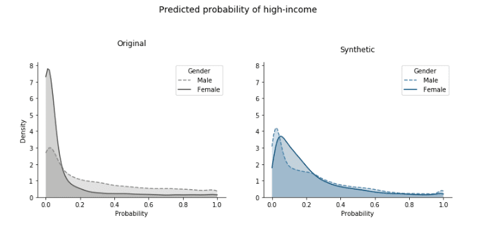
On the other hand, with the predictors trained on the synthetic data these distributions are brought very close together. This is exactly the group fairness that parity is designed to capture. The important thing to keep in mind though is that the predictive-model training itself did not involve any type of optimization to fairness and the evaluation is also on the biased original data. So this fair outcome is solely due to using bias-corrected synthetic data for the training.
Our results align with the findings of research conducted at Carnegie Mellon University into fair representations of data. We see that our fairness-constrained synthetic data solution learns to represent data points in a way that removes the dependencies between the sensitive and target attribute while preserving other relationships.
Correcting the Compas Data Set
We return briefly to the ProPublica study on algorithmic justice and the corresponding Compas data set (see our introductory fairness post). This data set contains information about defendants together with their predicted risk to re-offend, the so-called Compas score. We generate a parity-fair synthetic version of this data set with “race” as the sensitive attribute and the Compas score as the target variable. The original data set is heavily biased towards African Americans which in turn gets perfectly corrected in our synthetic data.
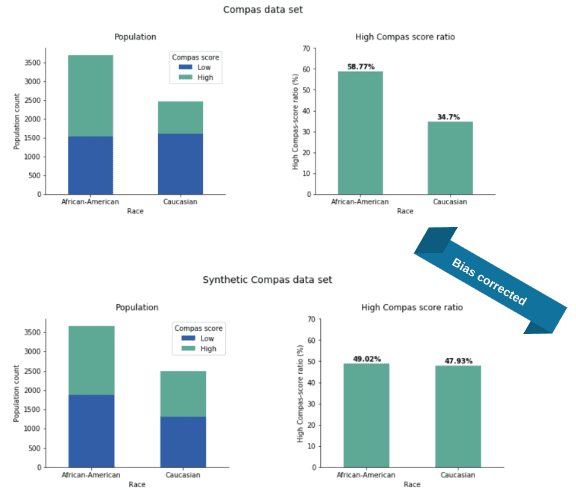
In the original Compas data set, the ratio of individuals with high Compas scores is 59% and 35% for African Americans and Caucasians, respectively. Quite impressively, our bias mitigated data reduced this gap to merely 1%, settling the values in the middle at 49% and 48%, respectively.
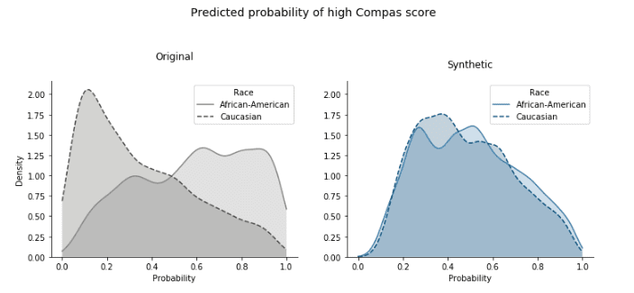
In the subsequent prediction task, we can achieve almost perfect equality between the predicted probabilities for high Compas score between the two classes of the sensitive attribute “race” (Figure 13).
Looking at the classifier’s performance, this parity-correction comes with minimal compromise in predictive accuracy (Figure 14).
Alternative Fairness Definitions
While demographic parity is a very intuitive notion, it has certain limitations. As compared to other fairness definitions, there is a worse trade-off between satisfying parity and having high accuracy for the generated data. If your original data had a class imbalance then the parity-mitigated synthetic data or a classifier that is forced to satisfy parity cannot achieve the same level of accuracy as a predictor with no parity loss. Actually, the base-rate difference is a provable lower bound on the accuracy. Moreover, parity is a notion of group fairness, it equalizes outcomes across classes, while other approaches optimize for individual fairness focusing on treating similar individuals similarly. S. Corbett-Davies and S. Goel argue that all these approaches suffer from serious shortcomings and advocate a risk-based assessment that could better serve policymaking.
Since parity only considers the sensitive attribute and a single other variable, it is not designed to handle a situation involving both predictions and a ground-truth label (three variables all together). So, in a more nuanced approach to fairness, one aims to have a predictor model that makes the same mistakes with the same chance across the sensitive attribute classes.
Such notions include equal opportunity and equalized odds which we also tested in our synthesis process: our experiments showed that if we generate synthetic data sets with these fairness constraints then they also give rise to fair classifiers with respect to these stronger notions. We will share the details of these more technical results in a subsequent article.
Conclusions and How We Will Continue After #FairnessWeek
The notion of fairness (in particular, statistical parity) and synthetic data go together very well. Not only can we generate highly accurate synthetic data but we can also steer the generation to almost perfectly mitigate strong biases in the original data sets. The additional fairness constraint in the training loss of our generative models fine-tunes the correlation structure between attributes such that these biases are strongly reduced. Privacy and (parity) fairness are further preserved in downstream tasks: an out-of-the-box classifier model when trained on fair synthetic data makes fair predictions even on biased input.
Statistical parity has limitations, and, on a more general note, there is no concept of fairness or silver-bullet solution that is applicable to all possible use cases. While this was our last post of #FairnessWeek, we will definitely continue our work on fair synthetic data and mitigating bias in Artificial Intelligence. In an upcoming study, we will extend our approach to other fairness measures, such as equal false-positivity rate and equalized odds.