In this tutorial, you will learn how to build a machine-learning model that is trained to distinguish between synthetic (fake) and real data records. This can be a helpful tool when you are given a hybrid dataset containing both real and fake records and want to be able to distinguish between them. Moreover, this model can serve as a quality evaluation tool for any synthetic data you generate. The higher the quality of your synthetic data records, the harder it will be for your ML discriminator to tell these fake records apart from the real ones.

You will be working with the UCI Adult Income dataset. The first step will be to synthesize the original dataset. We will start by intentionally creating synthetic data of lower quality in order to make it easier for our “Fake vs. Real” ML classifier to detect a signal and tell the two apart. We will then compare this against a synthetic dataset generated using MOSTLY AI's default high-quality settings to see whether the ML model can tell the fake records apart from the real ones.

The Python code for this tutorial is publicly available and runnable in this Google Colab notebook.

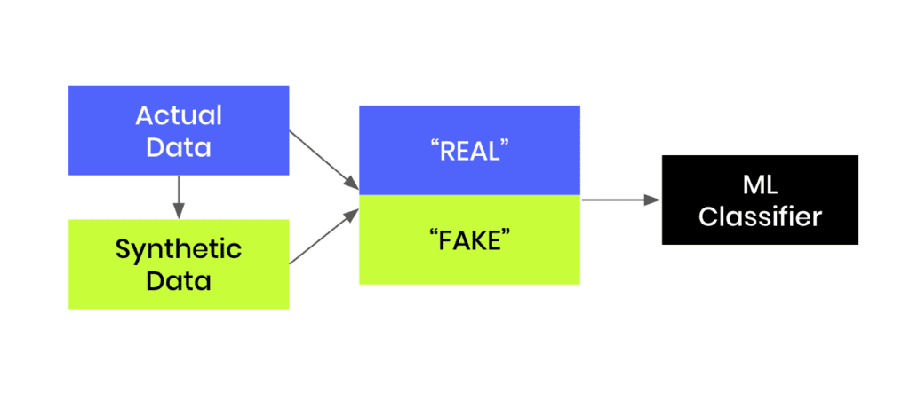
Fig 1 - Generate synthetic data and join this to the original dataset in order to train an ML classifier.

Create synthetic training data

Let’s start by creating our synthetic data:

1. Download the original dataset here. Depending on your operating system, use either Ctrl+S or Cmd+S to save the file locally. 

2. Go to your MOSTLY AI account and navigate to “Synthetic Datasets”. Upload the CSV file you downloaded in the previous step and click “Proceed”.

3. Set the Training Size to 1000. This will intentionally lower the quality of the resulting synthetic data. Click “Create a synthetic dataset” to launch the job.

Fig 2 - Set the Training Size to 1000.

4. Once the synthetic data is ready, download it to disk as CSV and use the following code to upload it if you’re running in Google Colab or to access it from disk if you are working locally:

# upload synthetic dataset
import pandas as pd

try:
    # check whether we are in Google colab
    from google.colab import files

    print("running in COLAB mode")
    repo = "https://github.com/mostly-ai/mostly-tutorials/raw/dev/fake-or-real"
    import io

    uploaded = files.upload()
    syn = pd.read_csv(io.BytesIO(list(uploaded.values())[0]))
    print(
        f"uploaded synthetic data with {syn.shape[0]:,} records"
        " and {syn.shape[1]:,} attributes"
    )
except:
    print("running in LOCAL mode")
    repo = "."
    print("adapt `syn_file_path` to point to your generated synthetic data file")
    syn_file_path = "./census-synthetic-1k.csv"
    syn = pd.read_csv(syn_file_path)
    print(
        f"read synthetic data with {syn.shape[0]:,} records"
        " and {syn.shape[1]:,} attributes"
    )

Train your “fake vs real” ML classifier

Now that we have our low-quality synthetic data, let’s use it together with the original dataset to train a LightGBM classifier. 

The first step will be to concatenate the original and synthetic datasets together into one large dataset. We will also create a split column to label the records: the original records will be labeled as REAL and the synthetic records as FAKE.

# concatenate FAKE and REAL data together
tgt = pd.read_csv(f"{repo}/census-49k.csv")
df = pd.concat(
    [
        tgt.assign(split="REAL"),
        syn.assign(split="FAKE"),
    ],
    axis=0,
)
df.insert(0, "split", df.pop("split"))

Sample some records to take a look at the complete dataset:

df.sample(n=5)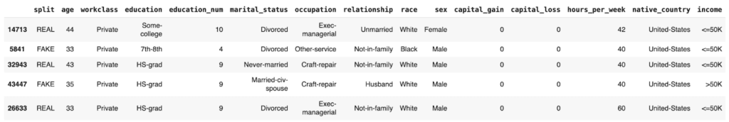

We see that the dataset contains both REAL and FAKE records.

By grouping by the split column and verifying the size, we can confirm that we have an even split of synthetic and original records:

df.groupby('split').size()

split 
FAKE 48842 
REAL 48842 
dtype: int64

The next step will be to train your LightGBM model on this complete dataset. The following code contains two helper scripts to preprocess the data and train your model:

import lightgbm as lgb
from lightgbm import early_stopping
from sklearn.model_selection import train_test_split

def prepare_xy(df, target_col, target_val):
    # split target variable `y`
    y = (df[target_col] == target_val).astype(int)
    # convert strings to categoricals, and all others to floats
    str_cols = [
        col
        for col in df.select_dtypes(["object", "string"]).columns
        if col != target_col
    ]
    for col in str_cols:
        df[col] = pd.Categorical(df[col])
    cat_cols = [
        col
        for col in df.select_dtypes("category").columns
        if col != target_col
    ]
    num_cols = [
        col for col in df.select_dtypes("number").columns if col != target_col
    ]
    for col in num_cols:
        df[col] = df[col].astype("float")
    X = df[cat_cols + num_cols]
    return X, y

def train_model(X, y):
    cat_cols = list(X.select_dtypes("category").columns)
    X_trn, X_val, y_trn, y_val = train_test_split(
        X, y, test_size=0.2, random_state=1
    )
    ds_trn = lgb.Dataset(
        X_trn, label=y_trn, categorical_feature=cat_cols, free_raw_data=False
    )
    ds_val = lgb.Dataset(
        X_val, label=y_val, categorical_feature=cat_cols, free_raw_data=False
    )
    model = lgb.train(
        params={"verbose": -1, "metric": "auc", "objective": "binary"},
        train_set=ds_trn,
        valid_sets=[ds_val],
        callbacks=[early_stopping(5)],
    )
    return model

Before training, make sure to set aside a holdout dataset for evaluation. Let’s reserve 20% of the records for this:

trn, hol = train_test_split(df, test_size=0.2, random_state=1)

Now train your LightGBM classifier on the remaining 80% of the combined original and synthetic data:

X_trn, y_trn = prepare_xy(trn, 'split', 'FAKE')
model = train_model(X_trn, y_trn)

Training until validation scores don't improve for 5 rounds 
Early stopping, best iteration is: 
[30] valid_0's auc: 0.594648

Next, score the model’s performance on the holdout dataset. We will include the model’s predicted probability for each record. A score of 1.0 indicates that the model is fully certain that the record is FAKE. A score of 0.0 means the model is certain the record is REAL.

Let’s sample some random records to take a look:

hol.sample(n=5)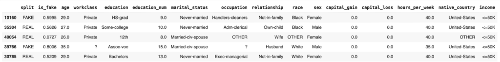

We see that the model assigns varying levels of probability to the REAL and FAKE records. In some cases it is not able to predict with much confidence (scores around 0.5) and in others it is  quite confident and also correct: see the 0.0727 for a REAL record and 0.8006 for a FAKE record.

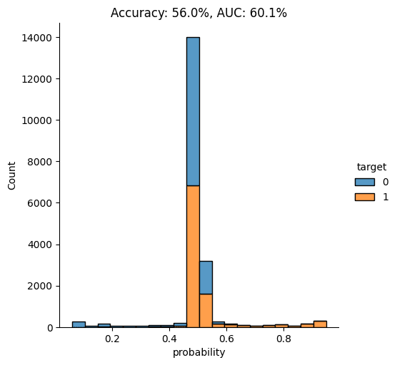
Let’s visualize the model’s overall performance by calculating the AUC and Accuracy scores and plotting the probability scores:

import seaborn as sns
import matplotlib.pyplot as plt
from sklearn.metrics import roc_auc_score, accuracy_score


auc = roc_auc_score(y_hol, hol.is_fake)
acc = accuracy_score(y_hol, (hol.is_fake > 0.5).astype(int))
probs_df = pd.concat(
    [
        pd.Series(hol.is_fake, name="probability").reset_index(drop=True),
        pd.Series(y_hol, name="target").reset_index(drop=True),
    ],
    axis=1,
)
fig = sns.displot(
    data=probs_df, x="probability", hue="target", bins=20, multiple="stack"
)
fig = plt.title(f"Accuracy: {acc:.1%}, AUC: {auc:.1%}")
plt.show()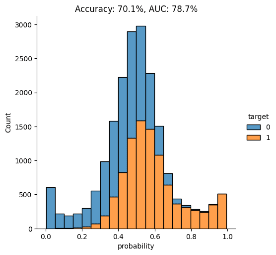

As you can see from the chart above, the discriminator has learned to pick up some signals that allow it with a varying level of confidence to determine whether a record is FAKE or REAL. The AUC can be interpreted as the percentage of cases in which the discriminator is able to correctly spot the FAKE record, given a set of a FAKE and a REAL record.

Let’s dig a little deeper by looking specifically at records that seem very fake and records that seem very real. This will give us a better understanding of the type of signals the model is learning.

Go ahead and sample some random records which the model has assigned a particularly high probability of being FAKE:

hol.sort_values('is_fake').tail(n=100).sample(n=5)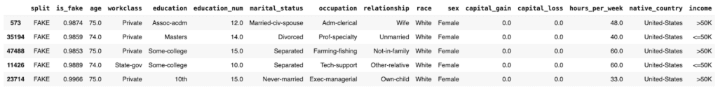

In these cases, it seems to be the mismatch between the education and education_num columns that gives away the fact that these are synthetic records. In the original data, these two columns have a 1:1 mapping of numerical to textual values. For example, the education value Some-college is always mapped to the numerical education_num value 10.0. In this poor-quality synthetic data, we see that there are multiple numerical values for the Some-college value, thereby giving away the fact that these records are fake.

Now let’s take a closer look at records which the model is especially certain are REAL:

hol.sort_values('is_fake').head(n=100).sample(n=5)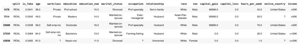

These “obviously real” records are types of records which the synthesizer has apparently failed to create. Thus, as they are then absent from the synthetic data, the discriminator recognizes these as REAL.

Generate high-quality synthetic data with MOSTLY AI

Now, let’s proceed to synthesize the original dataset again but this time using MOSTLY AI’s default settings for high-quality synthetic data. Run the same steps as before to synthesize the dataset except this time leave the Training Sample field blank. This will use all the records for the model training, ensuring the highest-quality synthetic data is generated. 

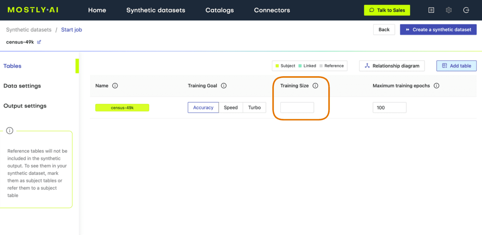
Fig 3 - Leave the Training Size blank to train on all available records.

Once the job has completed, download the high-quality data as CSV and then upload it to wherever you are running your code. 

Make sure that the syn variable now contains the new, high-quality synthesized data. Then re-run the code you ran earlier to concatenate the synthetic and original data together, train a new LightGBM model on the complete dataset, and evaluate its ability to tell the REAL records from FAKE.

Again, let’s visualize the model’s performance by calculating the AUC and Accuracy scores and by plotting the probability scores:

This time, we see that the model’s performance has dropped significantly. The model is not really able to pick up any meaningful signal from the combined data and assigns the largest share of records a probability around the 0.5 mark, which is essentially the equivalent of flipping a coin.

This means that the data you have generated using MOSTLY AI’s default high-quality settings is so similar to the original, real records that it is almost impossible for the model to tell them apart. 

Classifying “fake vs real” records with MOSTLY AI

In this tutorial, you have learned how to build a machine learning model that can distinguish between fake (i.e. synthetic) and real data records. You have synthesized the original data using MOSTLY AI and evaluated the resulting model by looking at multiple performance metrics. By comparing the model performance on both an intentionally low-quality synthetic dataset and MOSTLY AI’s default high-quality synthetic data, you have seen firsthand that the synthetic data MOSTLY AI delivers is so statistically representative of the original data that a top-notch LightGBM model was practically unable to tell these synthetic records apart from the real ones.

If you are interested in comparing performance across various data synthesizers, you may want to check out our benchmarking article which surveys 8 different synthetic data generators.

What’s next?

In addition to walking through the above instructions, we suggest:

• measuring the Discriminator's AUC if more training samples are used,
• using a different dataset,
• using a different ML model for the discriminator, eg. a RandomForest model,
• generate synthetic data with MOSTLY using your own dataset,
• using a different synthesizer, eg. SynthCity, SDV, etc.

You can also head straight to the other synthetic data tutorials:

• Generate synthetic text data
• Explainable AI with synthetic data
• Perform conditional data generation
• Rebalancing your data for ML classification problems
• Optimize your training sample size for synthetic data accuracy