
In this tutorial, you will learn how to validate synthetic data quality by evaluating its performance on a downstream Machine Learning (ML) task. The method you will learn is commonly referred to as the Train-Synthetic-Test-Real (TSTR) evaluation.
In a nutshell, we will train two ML models (one on original training data and one on synthetic data) and compare the performance of these two models in order to assess how well the synthetic data retains the statistical patterns present in the original data. The Python code for this tutorial is runnable and publicly available in this Google Colab notebook.
The TSTR evaluation serves as a robust measure of synthetic data quality because ML models rely on the accurate representation of deeper underlying patterns to perform effectively on previously unseen data. As a result, this approach offers a more reliable assessment than simply evaluating higher-level statistics.
The train-synthetic-test-real methodology
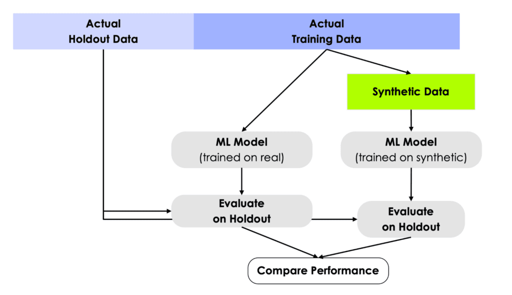
The TSTR method can be broken down into 5 steps:
- We start with an actual (real) data source and split this into a main dataset for training and a holdout dataset for evaluation.
- Next, we create a synthetic dataset only based on the training data.
- Then we train a Machine Learning (ML) model, and do so once using the synthetic data and once using the actual training data.
- We then evaluate the performance of each of these two models against the actual holdout data that was kept aside all along.
- By comparing the performance of these two models, we can assess how much utility has been retained by the synthesization method with respect to a specific ML task.
In the following sections, we will walk through each of these 5 steps using a real dataset and explain the Python code in detail.
This testing framework simulates the real-world scenario in which a model is trained on historical data but has to perform in production on data it has never seen before. For this reason, it’s crucial to use a true holdout dataset for the evaluation in order to properly measure out-of-sample performance.
1. Data prep
We will be working with a pre-cleaned version of the UCI Adult Income dataset, which itself stems from the 1994 American Community Survey by the US census bureau. The dataset consists of 48,842 records, 14 mixed-type features and has 1 target variable, that indicates whether a respondent had or had not reported a high level of annual income. We will use this dataset because it's one of the go-to datasets to showcase machine learning models in action.
The following code snippet can be used to split a DataFrame into a training and a holdout dataset.
from sklearn.model_selection import train_test_split

df = pd.DataFrame({'x': range(10), 'y': range(10, 20)})
df_trn, df_hol = train_test_split(df, test_size=0.2, random_state=1)
display(df_trn)
display(df_hol)
In the repo accompanying this tutorial, the data has already been split for you to save you some precious time 🙂
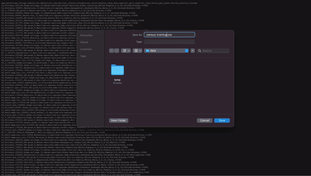
- Download the training data census-training.csv by clicking here and pressing Ctrl+S or Cmd+S to save the file locally. This is an 80% sample of the full dataset. The remaining 20% sample can be fetched from here.
2. Data synthesis
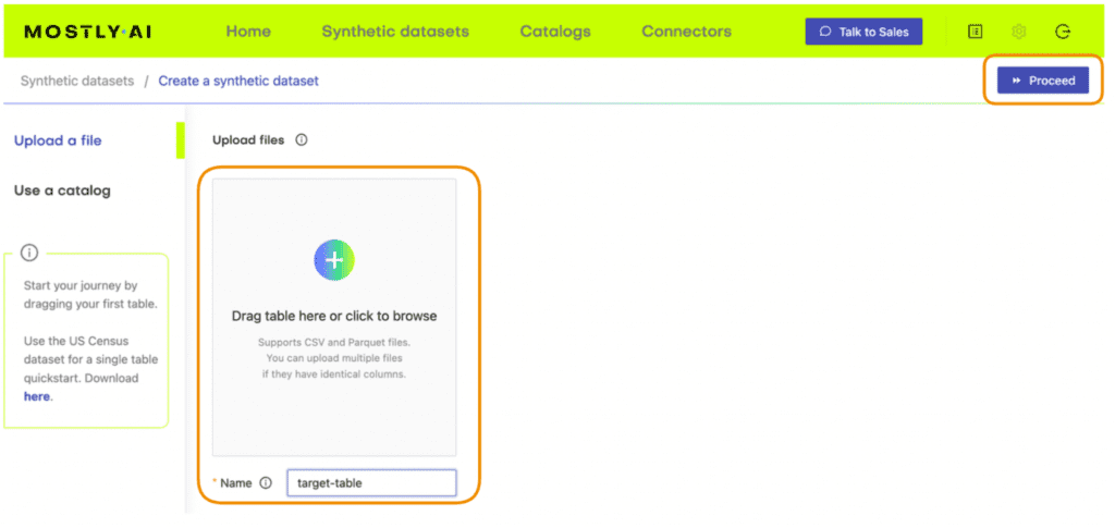
Next, we will create the synthesized version of the training dataset. Synthesize census-training.csv via MOSTLY AI's synthetic data generator by following the steps outlined below. You can leave all settings at their default, and just proceed to launch the job.
- Navigate to “Synthetic Datasets”. Upload census-training.csv and click “Proceed”.
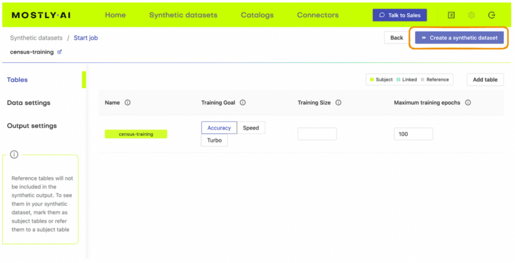
2. On the next page, click “Create a Synthetic Dataset” to launch the synthesization. You can leave all settings at their default.
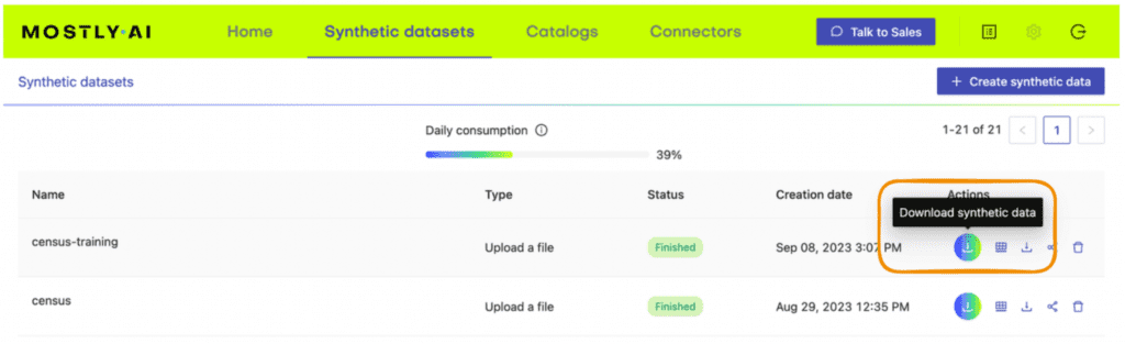
3. Follow the job’s progress using the UI and once the job has finished, download the generated synthetic data as CSV file to your computer. Optionally, you can also download a previously synthesized version here.
4. Return to your IDE or notebook and run the following code to create 3 DataFrames containing the training, synthesized and holdout data, respectively:
# upload synthetic dataset
import pandas as pd

try:
    # check whether we are in Google colab
    from google.colab import files
    print("running in COLAB mode")
    repo = 'https://github.com/mostly-ai/mostly-tutorials/raw/dev/train-synthetic-test-real'
    import io
    uploaded = files.upload()
    syn = pd.read_csv(io.BytesIO(list(uploaded.values())[0]))
    print(f"uploaded synthetic data with {syn.shape[0]:,} records and {syn.shape[1]:,} attributes")
except:
    print("running in LOCAL mode")
    repo = '.'
    print("adapt `syn_file_path` to point to your generated synthetic data file")
    syn_file_path = './census-synthetic.csv'
    syn = pd.read_csv(syn_file_path)
    print(f"read synthetic data with {syn.shape[0]:,} records and {syn.shape[1]:,} attributes")


# fetch training and holdout data
train = pd.read_csv(f'{repo}/census-training.csv')
print(f'fetched training data with {train.shape[0]:,} records and {train.shape[1]} attributes')
holdout = pd.read_csv(f'{repo}/census-holdout.csv')
print(f'fetched holdout data with {holdout.shape[0]:,} records and {holdout.shape[1]} attributes')
Before proceeding, let’s take a quick look at our freshly synthesized dataset by sampling 10 random records:
syn.sample(n=10)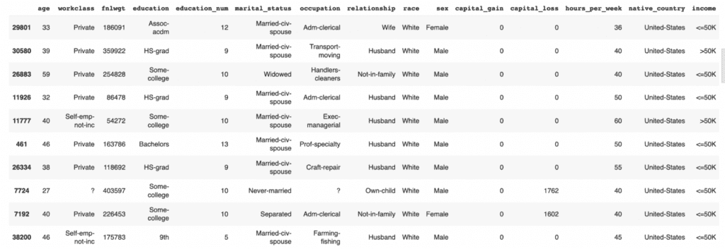
We can also get more specific by, for example, counting low-income and high-income records among the group of non-US citizens that have been divorced.
syn.loc[
    (syn["native_country"]!="United-States")
    & (syn["marital_status"]=="Divorced")
]['income'].value_counts()
<=50K 360
>50K 38
Name: income, dtype: int64Feel free to poke around the synthetic dataset more on your own to get a feel for the data.
3. ML training
Let's now train a state-of-the-art LightGBM classifier on top of the synthetic data, to then check how well it can predict whether an actual person reported an annual income of more than $50K or not. We will then compare the predictive accuracy to a model, that has been trained on the actual data, and see whether we were able to achieve a similar performance purely based on the synthetic data.
The following code block defines the target column and value and defines a function prepare_xy which preprocesses the data for ML training. The function casts the columns to the correct data types: columns containing strings are cast to categorical dtype and all numerical values are cast to float dtype. This is necessary for proper functioning of the LightGBM model. The function also splits the dataset into features X and target y.
Run the code block below to define the function.
# import necessary libraries
import lightgbm as lgb
from lightgbm import early_stopping
from sklearn.model_selection import train_test_split
from sklearn.metrics import roc_auc_score, accuracy_score
import seaborn as sns
import matplotlib.pyplot as plt

# define target column and value
target_col = 'income'
target_val = '>50K'

# define preprocessing function
def prepare_xy(df):
    y = (df[target_col]==target_val).astype(int)
    str_cols = [
        col for col in df.select_dtypes(['object', 'string'])
        .columns if col != target_col
    ]
    for col in str_cols:
        df[col] = pd.Categorical(df[col])
    cat_cols = [col for col in df.select_dtypes('category').columns if col != target_col]
    num_cols = [col for col in df.select_dtypes('number').columns if col != target_col]
    for col in num_cols:
        df[col] = df[col].astype('float')
    X = df[cat_cols + num_cols]
    return X, y
Now run the function prepare_xy to preprocess the data:
X_syn, y_syn = prepare_xy(syn)Next, we define a function train_model which will execute the ML training. The dataset is split into training and evaluation splits and the model is trained on the training dataset using some well-established base parameters. We specify early_stopping after 5 rounds without performance improvement in order to prevent overfitting.
3. Run the code block below to define the training function:
def train_model(X, y):
    cat_cols = list(X.select_dtypes('category').columns)
    X_trn, X_val, y_trn, y_val = train_test_split(X, y, test_size=0.2, random_state=1)
    ds_trn = lgb.Dataset(
        X_trn,
        label=y_trn,
        categorical_feature=cat_cols,
        free_raw_data=False
    )
    ds_val = lgb.Dataset(
        X_val,
        label=y_val,
        categorical_feature=cat_cols,
        free_raw_data=False
    )
    model = lgb.train(
        params={
            'verbose': -1,
            'metric': 'auc',
            'objective': 'binary'
        },
        train_set=ds_trn,
        valid_sets=[ds_val],
        callbacks=[early_stopping(5)],
    )
    return model
4. Now execute the training function:
model_syn = train_model(X_syn, y_syn)4. Synthetic data quality evaluation with ML
The next step is to evaluate the model’s performance on predicting the target feature y, which is whether or not a respondent had a high income. In this step we will be using the holdout dataset (which the model has never seen before) to evaluate the performance of the model trained on synthetic data: Train Synthetic, Test Real.
We’ll use two performance metrics:
- Accuracy: This is the probability to correctly predict the income class of a randomly selected record.
- AUC (Area-Under-Curve): This is the probability to correctly predict the income class, if two records, one of high-income and one of low-income are given.
Whereas the accuracy informs about the overall ability to get the class attribution correct, the AUC specifically informs about the ability to properly rank records, with respect to their probability of being within the target class or not. In both cases, the higher the metric, the better the predictive accuracy of the model.
We define a function evaluate_model which will perform the evaluation. This function first preprocesses the holdout data and then uses the model we have just trained on our synthetic data to try to predict the holdout dataset.
- Run the code block below to define the evaluation function:
def evaluate_model(model, hol):
    X_hol, y_hol = prepare_xy(hol)
    probs = model.predict(X_hol)
    preds = (probs >= 0.5).astype(int)
    auc = roc_auc_score(y_hol, probs)
    acc = accuracy_score(y_hol, preds)
    probs_df = pd.concat([
        pd.Series(probs, name='probability').reset_index(drop=True),
        pd.Series(y_hol, name=target_col).reset_index(drop=True)
    ], axis=1)
    sns.displot(
        data=probs_df,
        x='probability',
        hue=target_col,
        bins=20,
        multiple="stack"
    )
    plt.title(f"Accuracy: {acc:.1%}, AUC: {auc:.1%}", fontsize=20)
    plt.show()
    return auc
2. Now run the evaluation function:
auc_syn = evaluate_model(model_syn, holdout)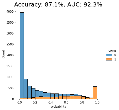
The displayed chart shows the distribution of scores that the model assigned to each of the holdout records. A score close to 0 means that model is very confident that the record is of low income. A score close to 1 means that the model is very confident that it's a high income record. These scores are further split by their actual outcome, i.e. whether they are or are not actually high income. This allows us to visually inspect the model's confidence in assigning the right scores.
We can see that the model trained on synthetic data seems to perform quite well when testing against real data it has never seen before (i.e. the holdout dataset). Both the accuracy and AUC scores give us confidence that this model may perform well in production.
But the real test is: how does the performance of this model trained on synthetic data compare against the performance of a model trained on real data? Remember: the purpose of this exercise is to discover whether we can use high-quality synthetic data to train our ML models instead of the original data (to protect data privacy) without losing significant predictive performance.
5. ML performance comparison
So let's now compare the results achieved on synthetic data with a model trained on real data. For a very good synthesizer, we expect to see a predictive performance of the two models being close to each other.
- Run the same 3 functions as we did above to prepare the data, train the model and evaluate it, but this time using the original dataset rather than the synthetic data:
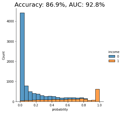
For the given dataset, and the given synthesizer, we can observe a near on-par performance of the synthetic data with respect to the given downstream ML task. Both accuracy scores are around 87% and both AUC scores are around 92%, with a maximum of 0.5% difference.
This means that in this case you can train your LightGBM machine learning model purely on synthetic data and be confident that it will yield equally performant results as if it were trained on real data, but without ever putting the privacy of any of the contained individuals at any risk.
What did we learn about synthetic data quality evaluations?
This tutorial has introduced you to the Train Synthetic Test Real methodology for synthetic data quality evaluations, specifically by measuring its utility on a downstream ML task. This evaluation method is more robust than only looking at high-level statistics because ML models rely on the accurate representation of deeper underlying patterns to perform effectively on previously unseen data.
By testing your model trained on synthetic data on a holdout dataset containing original (real) data that the model has never seen before, you can now effectively assess the quality of your synthesized datasets. With the right dataset, model and synthesizer, you can train your ML models entirely on synthetic data and be confident that you are getting maximum predictive power and privacy preservation.
What’s next?
In addition to walking through the above instructions, we suggest:
- to run the Train-Synthetic-Test-Real synthetic data quality evaluation
- using a different dataset, eg. the UCI bank-marketing dataset
- using a different downstream ML model, eg. a RandomForest model
- using a different synthesizer, eg. SynthCity, SDV, etc.
- to check the impact of synthetic upsampling by generating 10x or 100x the original data records, and see whether it improves ML accuracy.