In this tutorial, you will learn how to generate synthetic text using MOSTLY AI's synthetic data generator. While synthetic data generation is most often applied to structured (tabular) data types, such as numbers and categoricals, this tutorial will show you that you can also use MOSTLY AI to generate high-quality synthetic unstructured data, such as free text.

You will learn how to use the MOSTLY AI platform to synthesize text data and also how to evaluate the quality of the synthetic text that you will generate. For context, you may want to check out the introductory article which walks through a real-world example of using synthetic text when working with voice assistant data.

You will be working with a public dataset containing AirBnB listings in London. We will walk through how to synthesize this dataset and pay special attention to the steps needed to successfully synthesize the columns containing unstructured text data. We will then proceed to evaluate the statistical quality of the generated text data by inspecting things like the set of characters, the distribution of character and term frequencies and the term co-occurrence.

We will also perform a privacy check by scanning for exact matches between the original and synthetic text datasets. Finally, we will evaluate the correlations between the synthesized text columns and the other features in the dataset to ensure that these are accurately preserved. The Python code for this tutorial is publicly available and runnable in this Google Colab notebook.

Synthesize text data

Synthesizing text data with MOSTLY AI can be done through a single step before launching your data generation job. We will indicate which columns contain unstructured text and let MOSTLY AI’s generative algorithm do the rest.

Let’s walk through how this works:

1. Download the original AirBnB dataset. Depending on your operating system, use either Ctrl+S or Cmd+S to save the file locally. 

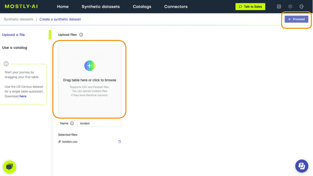
2. Go to your MOSTLY AI account and navigate to “Synthetic Datasets”. Upload the CSV file you downloaded in the previous step and click “Proceed”.

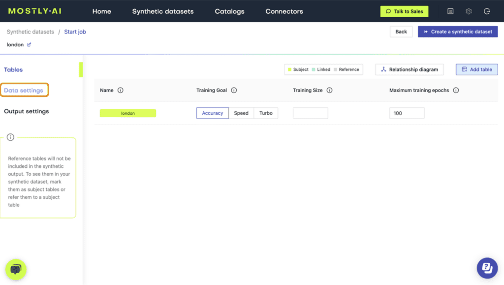
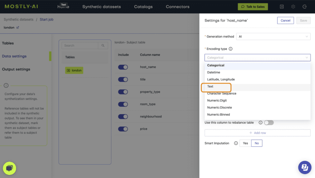
3. Navigate to “Data Settings” in order to specify which columns should be synthesized as unstructured text data.

4. Click on the host_name and title columns and set the Generation Method to “Text”.

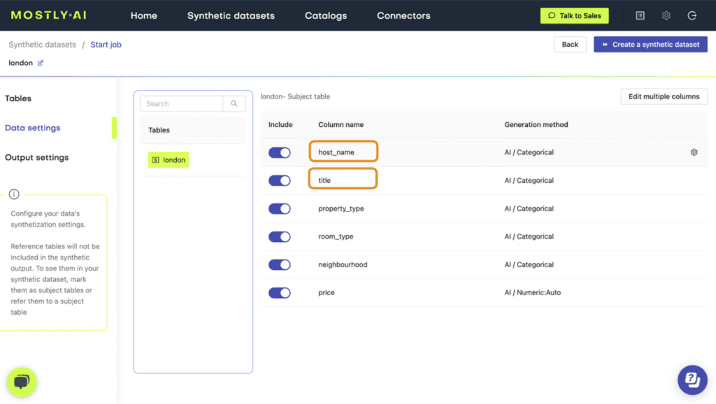
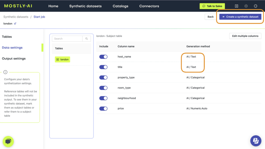
5. Verify that both columns are set to Generation Method “AI / Text” and then launch the job by clicking “Create a synthetic dataset”. Synthetic text generation is compute-intensive, so this may take up to an hour to complete.

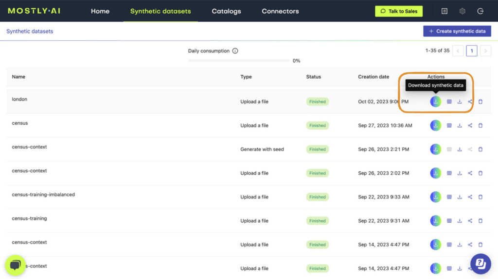
6. Once completed, download the synthetic dataset as CSV. 

And that’s it! You have successfully synthesized unstructured text data using MOSTLY AI.

You can now poke around the synthetic data you’ve created, for example, by sampling 5 random records:

syn.sample(n=5)

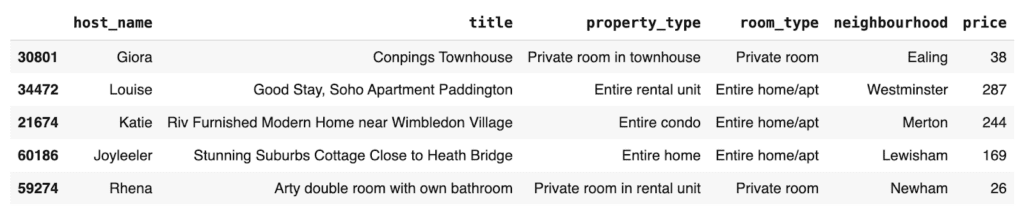
And compare this to 5 random records sampled from the original dataset:

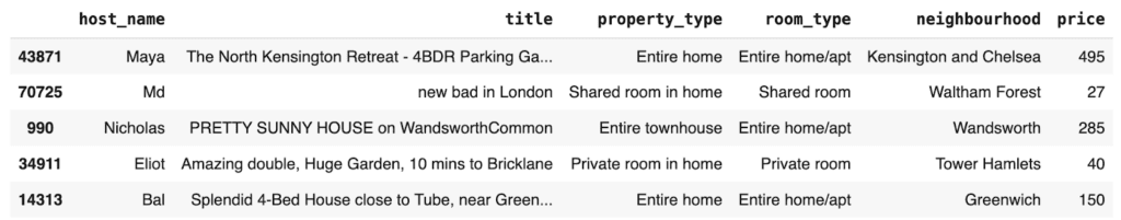
But of course, you shouldn’t just take our word for the fact that this is high-quality synthetic data. Let’s be a little more critical and evaluate the data quality in more detail in the next section. 

Evaluate statistical integrity

Let’s take a closer look at how statistically representative the synthetic text data is compared to the original text. Specifically, we’ll investigate four different aspects of the synthetic data: (1) the character set, (2) the character and (3) term frequency distributions, and (4) the term co-occurrence. We’ll explain the technical terms in each section.

Character set

Let’s start by taking a look at the set of all characters that occur in both the original and synthetic text. We would expect to see a strong overlap between the two sets, indicating that the same kinds of characters that appear in the original dataset also appear in the synthetic version.

The code below generates the set of characters for the original and synthetic versions of the title column:

print(
    "## ORIGINAL ##\n",
    "".join(sorted(list(set(tgt["title"].str.cat(sep=" "))))),
    "\n",
)
print(
    "## SYNTHETIC ##\n",
    "".join(sorted(list(set(syn["title"].str.cat(sep=" "))))),
    "\n",
)

The output is quite long and is best inspected by running the code in the notebook yourself. 

We see a perfect overlap in the character set for all characters up until the “£” symbol. These are all the most commonly used characters. This is a good first sign that the synthetic data contains the right kinds of characters.

From the “£” symbol onwards, you will note that the character set of the synthetic data is shorter. This is expected and is due to the privacy mechanism called rare category protection within the MOSTLY AI platform, which removes very rare tokens in order to prevent their presence giving away information on the existence of individual records in the original dataset.

Character frequency distribution

Next, let’s take a look at the character frequency distribution: how many times each letter shows up in the dataset. Again, we will compare this statistical property between the original and synthetic text data in the title column.

The code below creates a list of all characters that occur in the datasets along with the percentage that character constitutes of the whole dataset:

title_char_freq = (
    pd.merge(
        tgt["title"]
        .str.split("")
        .explode()
        .value_counts(normalize=True)
        .to_frame("tgt")
        .reset_index(),
        syn["title"]
        .str.split("")
        .explode()
        .value_counts(normalize=True)
        .to_frame("syn")
        .reset_index(),
        on="index",
        how="outer",
    )
    .rename(columns={"index": "char"})
    .round(5)
)
title_char_freq.head(10)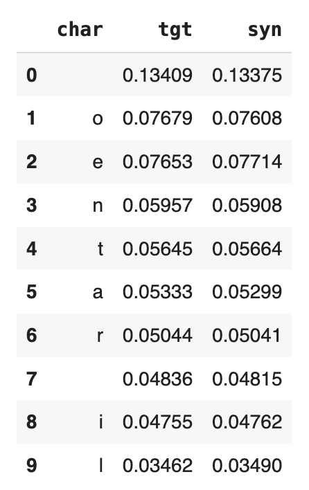

We see that “o” and “e” are the 2 most common characters (after the whitespace character), both showing up a little more than 7.6% of the time in the original dataset. If we inspect the syn column, we see that the percentages match up nicely. There are about as many “o”s and “e”s in the synthetic dataset as there are in the original now. And this goes for the other characters in the list as well. 

For a visualization of all the distributions of the 100 most common characters, you can run the code below:

import matplotlib.pyplot as plt
ax = title_char_freq.head(100).plot.line()
plt.title('Distribution of Char Frequencies')
plt.show()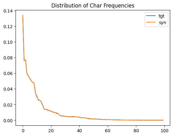

We see that the original distribution (in light blue) and the synthetic distribution (orange) are almost identical. This is another important confirmation that the statistical properties of the original text data are being preserved during the synthetic text generation. 

Term frequency distribution

Let’s now do the same exercise we did above but with words (or “terms”) instead of characters. We will look at the term frequency distribution: how many times each term shows up in the dataset and how this compares across the synthetic and original datasets.

The code below performs some data cleaning and then performs the analysis and displays the 10 most frequently used terms.

import re

def sanitize(s):
    s = str(s).lower()
    s = re.sub('[\\,\\.\\)\\(\\!\\"\\:\\/]', " ", s)
    s = re.sub("[ ]+", " ", s)
    return s

tgt["terms"] = tgt["title"].apply(lambda x: sanitize(x)).str.split(" ")
syn["terms"] = syn["title"].apply(lambda x: sanitize(x)).str.split(" ")
title_term_freq = (
    pd.merge(
        tgt["terms"]
        .explode()
        .value_counts(normalize=True)
        .to_frame("tgt")
        .reset_index(),
        syn["terms"]
        .explode()
        .value_counts(normalize=True)
        .to_frame("syn")
        .reset_index(),
        on="index",
        how="outer",
    )
    .rename(columns={"index": "term"})
    .round(5)
)
display(title_term_freq.head(10))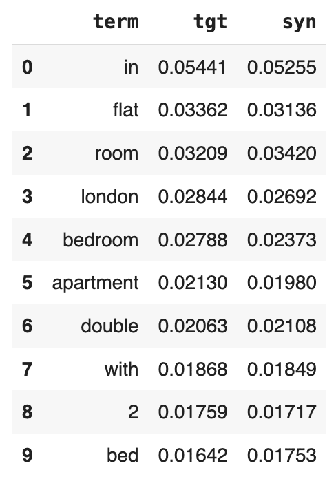

You can also take a look at the 10 least-common words:

display(title_term_freq.head(200).tail(10))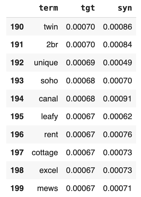

And again, plot the entire distribution for a comprehensive overview:

ax = title_term_freq.head(100).plot.line()
plt.title('Distribution of Term Frequencies')
plt.show()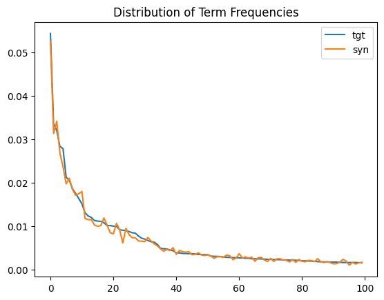

Just as we saw above with the character frequency distribution, we see a close match between the original and synthetic term frequency distributions. The statistical properties of the original dataset are being preserved.

Term co-occurrence

As a final statistical test, let’s take a look at the term co-occurrence: how often a word appears in a given listing title given the presence of another word. For example, how many words that contain the word “heart” also contain the word “London”?

The code below defines a helper function to calculate the term co-occurrence given two words:

def calc_conditional_probability(term1, term2):
    tgt_beds = tgt["title"][
        tgt["title"].str.lower().str.contains(term1).fillna(False)
    ]
    syn_beds = syn["title"][
        syn["title"].str.lower().str.contains(term1).fillna(False)
    ]
    tgt_beds_double = tgt_beds.str.lower().str.contains(term2).mean()
    syn_beds_double = syn_beds.str.lower().str.contains(term2).mean()
    print(
        f"{tgt_beds_double:.0%} of actual Listings, that contain `{term1}`, also contain `{term2}`"
    )
    print(
        f"{syn_beds_double:.0%} of synthetic Listings, that contain `{term1}`, also contain `{term2}`"
    )
    print("")

Let’s run this function for a few different examples of word combinations:

calc_conditional_probability('bed', 'double')
calc_conditional_probability('bed', 'king')
calc_conditional_probability('heart', 'london')
calc_conditional_probability('london', 'heart')

14% of actual Listings, that contain `bed`, also contain `double` 

13% of synthetic Listings, that contain `bed`, also contain `double` 

7% of actual Listings, that contain `bed`, also contain `king` 

6% of synthetic Listings, that contain `bed`, also contain `king` 

28% of actual Listings, that contain `heart`, also contain `london` 

26% of synthetic Listings, that contain `heart`, also contain `london` 

4% of actual Listings, that contain `london`, also contain `heart` 

4% of synthetic Listings, that contain `london`, also contain `heart`

Once again, we see that the term co-occurrences are being accurately preserved (with some minor variation) during the process of generating the synthetic text.

Now you might be asking yourself: if all of these characteristics are maintained, what are the chances that we'll end up with exact matches, i.e., synthetic records with the exact same title value as a record in the original dataset? Or perhaps even a synthetic record with the exact same values for all the columns?

Let's start by trying to find an exact match for 1 specific synthetic title value. Choose a title_value from the original title column and then use the code below to search for an exact match in the synthetic title column.

title_value = "Airy large double room"
tgt.loc[tgt["title"].str.contains(title_value, case=False, na=False)]

We see that there is an exact (partial) match in this case. Depending on the value you choose, you may or may not find an exact match. But how big of a problem is it that we find an exact partial match? Is this a sign of a potential privacy breach? It’s hard to tell from a single row-by-row validation, and, more importantly, this process doesn't scale very well to the 71K rows in the dataset.

Evaluate the privacy of synthetic text

Let's perform a more comprehensive check for privacy by looking for exact matches between the synthetic and the original.

To do that, first split the original data into two equally-sized sets and measure the number of matches between those two sets:

n = int(tgt.shape[0]/2)
pd.merge(tgt[['title']][:n].drop_duplicates(), tgt[['title']][n:].drop_duplicates())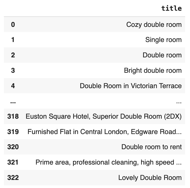

This is interesting. There are 323 cases of duplicate title values in the original dataset itself. This means that the appearance of one of these duplicate title values in the synthetic dataset would not point to a single record in the original dataset and therefore does not constitute a privacy concern.

What is important to find out here is whether the number of exact matches between the synthetic dataset and the original dataset exceeds the number of exact matches within the original dataset itself. 

Let’s find out.

Take an equally-sized subset of the synthetic data, and again measure the number of matches between that set and the original data:

pd.merge(
    tgt[["title"]][:n].drop_duplicates(), syn[["title"]][:n].drop_duplicates()
)

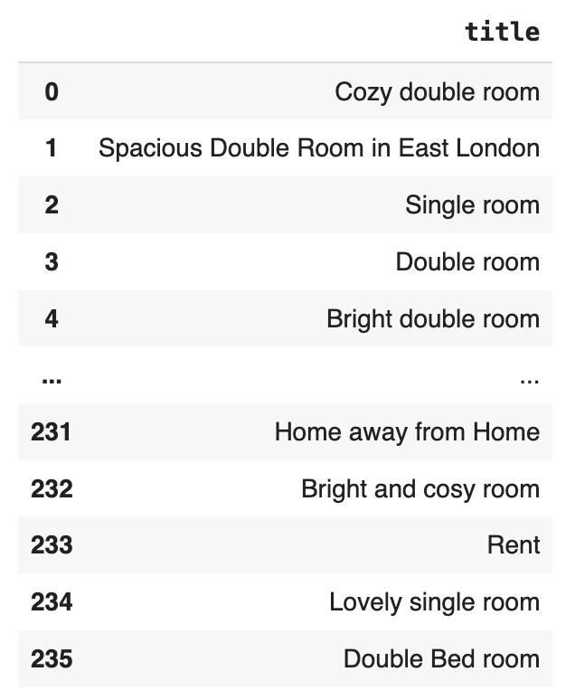
There are 236 exact matches between the synthetic dataset and the original, but significantly less than the number of exact matches that exist within the original dataset itself. Moreover, we can see that they occur only for the most commonly used descriptions.

It’s important to note that matching values or matching complete records are by themselves not a sign of a privacy leak. They are only an issue if they occur more frequently than we would expect based on the original dataset. Also note that removing those exact matches via post-processing would actually have a detrimental contrary effect. The absence of a value like "Lovely single room" in a sufficiently large synthetic text corpus would, in this case, actually give away the fact that this sentence was present in the original. See our peer-reviewed academic paper for more context on this topic.

Correlations between text and other columns

So far, we have inspected the statistical quality and privacy preservation of the synthesized text column itself. We have seen that both the statistical properties and the privacy of the original dataset are carefully maintained.

But what about the correlations that exist between the text columns and other columns in the dataset? Are these correlations also maintained during synthesization?

Let’s take a look by inspecting the relationship between the title and price columns. Specifically, we will look at the median price of listings that contain specific words that we would expect to be associated with a higher (e.g., “luxury”) or lower (e.g., “small”) price. We will do this for both the original and synthetic datasets and compare.

The code below prepares the data and defines a helper function to print the results:

tgt_term_price = (
    tgt[["terms", "price"]]
    .explode(column="terms")
    .groupby("terms")["price"]
    .median()
)
syn_term_price = (
    syn[["terms", "price"]]
    .explode(column="terms")
    .groupby("terms")["price"]
    .median()
)

def print_term_price(term):
    print(
        f"Median Price of actual Listings, that contain `{term}`: ${tgt_term_price[term]:.0f}"
    )
    print(
        f"Median Price of synthetic Listings, that contain `{term}`: ${syn_term_price[term]:.0f}"
    )

print("")

Let’s then compare the median price for specific terms across the two datasets:

print_term_price("luxury")
print_term_price("stylish")
print_term_price("cozy")
print_term_price("small")

Median Price of actual Listings, that contain `luxury`: $180 
Median Price of synthetic Listings, that contain `luxury`: $179 

Median Price of actual Listings, that contain `stylish`: $134 
Median Price of synthetic Listings, that contain `stylish`: $140 

Median Price of actual Listings, that contain `cozy`: $70 
Median Price of synthetic Listings, that contain `cozy`: $70 

Median Price of actual Listings, that contain `small`: $55 
Median Price of synthetic Listings, that contain `small`: $60

We can see that correlations between the text and price features are very well retained.

Generate synthetic text with MOSTLY AI

In this tutorial, you have learned how to generate synthetic text using MOSTLY AI by simply specifying the correct Generation Method for the columns in your dataset that contain unstructured text. You have also taken a deep dive into evaluating the statistical integrity and privacy preservation of the generated synthetic text by looking at character and term frequencies, term co-occurrence, and the correlations between the text column and other features in the dataset. These statistical and privacy indicators are crucial components for creating high-quality synthetic data.

What’s next?

In addition to walking through the above instructions, we suggest experimenting with the following in order to get even more hands-on experience generating synthetic text data:

• analyzing further correlations, also for host_name
• using a different generation mood, e.g., conservative sampling. Take a look at the end of the video tutorial for a quick walkthrough.
• using a different dataset, e.g., the Austrian First Name dataset

You can also head straight to the other synthetic data tutorials:

• Evaluate synthetic data quality using downstream ML
• Optimize your training sample size for synthetic data accuracy
• Rebalancing your data for ML classification problems
• Perform conditional data generation
• Explainable AI with synthetic data
• How to generate synthetic data