What is time series data?
Time series data is a sequence of data points that are collected or recorded at intervals over a period of time. What makes a time series dataset unique is the sequence or order in which these data points occur. This ordering is vital to understanding any trends, patterns, or seasonal variations that may be present in the data.
In a time series, data points are often correlated and dependent on previous values in the series. For example, when a financial stock price moves every fraction of a second, its movements are based on previous positions and trends. Time series data becomes a valuable asset in predicting future values based on these past patterns, a process known as forecasting.
Time series forecasting employs specialized statistical techniques to effectively model and generate future predictions. It is commonly used in business, finance, environmental science, and many other areas for decision-making and strategic planning.
Types of time series data
Time series data can be categorized in various ways, each with its own characteristics and analytical approaches.
Metric-based time series data
When measurements are taken at regular intervals, these are known as time series metrics. Metrics are crucial for observing trends, detecting anomalies, and forecasting future values based on historical patterns.
This type of time series data is commonly seen in financial datasets, where stock prices are recorded at consistent intervals, or in environmental monitoring, where temperature, pressure, or humidity data is collected periodically.

Source: Unsplash
Event-based time series
Event-based time series data captures occurrences that happen at specific points in time, but not necessarily at regular intervals. While this data can still be aggregated into snapshots over traditional periods, the event-based time series data forms a more complex series of related activities.

Source: Unsplash
Examples include system logging in IT networks, where each entry records an event like a system error or a transaction. Electronic health records capture patient interactions with doctors, with medical devices capturing complex health telemetry over time. City-wide sensor networks capture the telemetry from millions of individual transport journeys, including bus, subway, and taxi routes.
Event-based data is vital to understanding the sequences and relationships between occurrences that help drive decision-making in cybersecurity, customer behavioral analysis, and many other domains.
Linear time series data
Time series data can also be categorized based on how the patterns within the time series behave over time. Linear time series data is more straightforward to model and forecast, with consistent behavior from one time period to the next.
Stock prices are a classic example of a linear time series. The value of a company’s shares is recorded at regular intervals, reflecting the latest market valuation. Analyzing this data over extended periods helps investors make informed decisions about buying and selling stocks based on historical performance and predicted trends.
Non-linear time series data
In contrast, non-linear time series data is often more complex, with changes that do not follow a predictable pattern. Such time series are often found in more dynamic systems when external factors force changes in behavior that may be short-lived.
For example, short-term demand modeling for public transport after an event or incident will likely follow a complex pattern that combines the time of day, geolocation information, and other factors, making reliable predictions more complicated. With IoT wearables for health, athletes are constantly monitored for early warning signals of injury or fatigue. These data points do not follow a traditional linear time series model; instead, they require a broader range of inputs to assess and predict areas of concern.
Behavioral time series data
Capturing time series data around user interactions or consumer patterns produces behavioral datasets that can provide insights into habits, preferences, or individual decisions. Behavioral time series data is becoming increasingly important to social scientists, designers, and marketers to better understand and predict human behavior in various contexts.
From measuring whether daily yoga practice can impact device screen time habits to analyzing over 285 million user events from an eCommerce website, behavioral time series data can exist as either metrics- or event-based time series datasets.
Metrics-based behavioral analytics are widespread in financial services, where customer activity over an extended period is used to assess suitability for loans or other services. Event-based behavioral analytics are often deployed as prescriptive analytics against sequences of events that represent transactions, visits, clicks, or other actions.
Organizations use behavioral analytics at scale to provide customers visiting websites, applications, or even brick-and-mortar stores with a “next best action” that will add value to their experience.
Despite the immense growth of behavioral data captured through digital transformation and investment programs, there are still major challenges to driving value from this largely untapped data asset class.
Since behavioral data typically stores thousands of data points per customer, individuals are increasingly likely to be re-identified, resulting in privacy breaches. Legacy data anonymization techniques, such as data masking, fail to provide strong enough privacy controls or remove so much from the data that it loses its utility for analytics altogether.
Examples of time series data
Let’s explore some common examples of time series data from public sources.
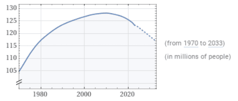
From the US Federal Reserve, a data platform known as the Federal Reserve Economic Database (FRED) collects time series data related to populations, employment, socioeconomic indicators, and many more categories.
Some of FRED’s most popular time series datasets include:
| Category | Source | Frequency | Data Since |
|---|---|---|---|
| Population | US Bureau of Economic Analysis | Monthly | 1959 |
| Employment (Nonfarm Private Payroll) | Automatic Data Processing, Inc. | Weekly | 2010 |
| National Accounts (Federal Debt) | US Department of the Treasury | Quarterly | 1966 |
| Environmental (Jet Fuel CO2 Emissions) | US Energy Information Administration | Annually | 1973 |
Beyond socioeconomic and political indicators, time series data plays a critical role in the decision-making processes behind financial services, especially banking activities such as trading, asset management, and risk analysis.
| Category | Source | Frequency | Data Since |
|---|---|---|---|
| Interest Rates (e.g., 3-Month Treasury Bill Secondary Market Rates) | Federal Reserve | Daily | 2018 |
| Exchange Rates (e.g., USD to EUR Spot Exchange Rate) | Federal Reserve | Daily | 2018 |
| Consumer Behavior (e.g., Large Bank Consumer Credit Card Balances) | Federal Reserve Bank of Philadelphia | Quarterly | 2012 |
| Markets Data (e.g., commodities, futures, equities, etc.) | Bloomberg, Reuters, Refinitiv, and many others | Real-Time | N/A |
The website kaggle.com provides an extensive repository of publicly available datasets, many recorded as time series.
| Category | Source | Frequency | Data Range |
|---|---|---|---|
| Environmental (Jena Climate Dataset) | Max Planck Institute for Biogeochemistry | Every 10 minutes | 2009-2016 |
| Transportation (NYC Yellow Taxi Trip Data) | NYC Taxi & Limousine Commission (TLC) | Monthly updates, with individual trip records | 2009- |
| Public Health (COVID-19) | World Health Organization | Daily | 2020- |
An emerging category of time series data relates to the growing use of Internet of things (IoT) devices that capture and transmit information for storage and processing. IoT devices, such as smart energy meters, have become extremely popular in both industrial applications (e.g., manufacturing sensors) and commercial use.
| Category | Source | Frequency | Data Range |
|---|---|---|---|
| IoT Consumer Energy (Smart Meter Telemetry) | Jaganadh Gopinadhan (Kaggle) | Minute | 12-month period |
| IoT Temperature Measurements | Atul Anand (Kaggle) | Second | 12-month period |
How to store time series data
Once time series data has been captured, there are several popular options for storing, processing, and querying these datasets using standard components in a modern data stack or via more specialist technologies.
File formats for time series data
Storing time series data in file formats like CSV, JSON, and XML is common due to their simplicity and broad compatibility. With CSV files especially, this makes them ideal for smaller datasets, where ease of use and portability are critical.
Formats such as Parquet have become increasingly popular for storing large-scale time series datasets, offering efficient compression and high performance for analysis. However, Parquet can be more complex and resource-intensive than simpler file formats, and managing large numbers of Parquet files, especially in a rapidly changing time series context, can become challenging.
When more complex data structures are involved, JSON and XML formats provide a structured way to store time series data, complete with associated metadata, especially when using APIs to transfer information between systems. JSON and XML typically require additional processing to “flatten” the data for analysis and are not ideal for large datasets.
For most time series stored in files, it’s recommended to use the more straightforward CSV format where possible, switching to Parquet when data volumes affect storage efficiency and read/write speeds, typically at the gigabyte or terabyte scale. Likewise, a synthetically generated time series can be easily exported to tabular CSV or Parquet format for downstream analysis in various tools.
Time series databases
Dedicated time series databases, such as Kx Systems, are specifically designed to manage and analyze sequences of data points indexed over time. These databases are optimized for handling large volumes of data that are constantly changing or being updated, making them ideal for applications in financial markets such as high-frequency trading, IoT sensor data, or real-time monitoring.
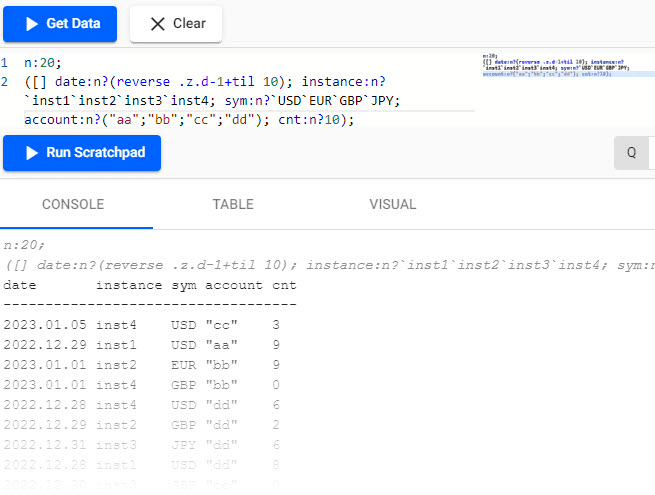
Source: Kx query
Graph databases for time series
Graph databases like Neo4j offer a unique approach to storing time series data by representing it as a network of interconnected nodes and relationships. Graph databases allow for the modeling of complex relationships, providing insights that might be difficult to extract from traditional relational data models.
The ability to explore relationships efficiently in graph databases makes them suitable for analyses that require a deep understanding of interactions over time, adding a rich layer of context to the time series data.
In the example below, Neo4j can create a “TimeTree” graph data model that captures events used in risk and compliance analysis. Exploring emails sent at different times to different parties and any associated events from that period becomes possible.
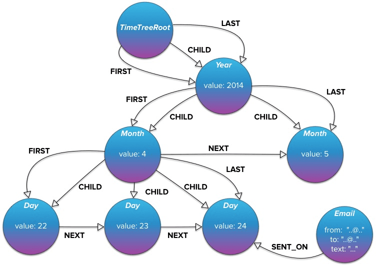
Source: Neo4j time-tree
Relational databases for time series
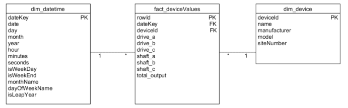
For decades, traditional relational database management systems (RDBMS) like Snowflake, Postgres, or Redshift have been used to store, process, and analyze time series data. One of the most popular relational data models for time series analysis is known as the star schema, where a central fact table (containing the time series data such as events, transactions, or behaviors) is connected to several dimension tables (e.g., customer, store, product, etc.) that provide rich analytical context.
By capturing events at a granular level, the time series data can be sliced and diced in many different ways, giving analysts a great deal of flexibility to answer questions and explore business performance. Usually, a date dimension table contains all the relevant context for a time series analysis, with attributes such as day of the week, month, and quarter, as well as valuable references to prior periods for comparison.
In a well-designed star schema model, the number of dimensions associated with a transactional fact table generally ranges between six and 15. These dimensions, which provide the contextual details necessary to understand and analyze the facts, depend on the specific analysis needs and the complexity of the business domain. MOSTLY AI can generate highly realistic synthetic data that fully retains the correlations from the original dimensions and fact tables across star schema data models with three or more entities.
Source: Stack Exchange
How to analyze time series data
Before analyzing a time series model, there are several essential terms and concepts to review.
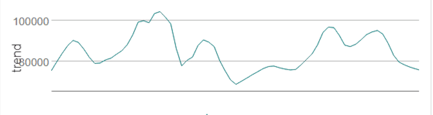
Trend
A trend is a long-term value increase or decrease within a time series. Trends do not have to be linear and may reverse direction over time.
Source: WolframAlpha
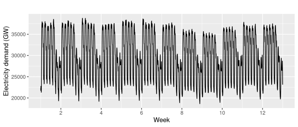
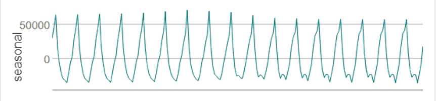
Seasonality
Seasonality is a pattern that occurs in a time series dataset at a fixed interval, such as the time of year or day of the week. Most commonly associated with physical properties such as temperature or rainfall, seasonality is also applied to consumer behavior driven by public holidays or promotional events.
Data retention over extended periods allows analysts to observe long-term patterns and variations. This historical perspective is essential for distinguishing between one-time anomalies and consistent seasonal fluctuations, providing valuable insights for forecasting and strategic planning.

Adapted from: Climates to Travel
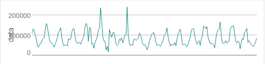
Cyclicity
A cyclic pattern occurs when observations rise and fall at non-fixed frequencies. Often, cycles last for multiple years, but the cyclic duration can only sometimes be determined in advance.
Source: Rob J. Hyndman
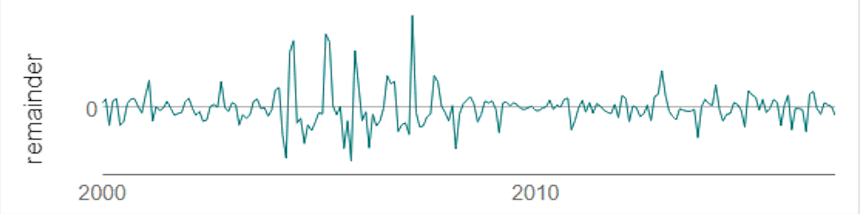
Random noise
The final component to a time series is random noise, once any trends, seasonality, or cyclic signals have been accounted for. Any time series that contains too much random noise will be challenging to forecast or analyze.
Preparing data for time series analysis: Fill the gaps
Once a time series dataset has been collected, ensuring no missing dates within the sequence is vital. Review the granularity of the data set and impute any missing elements to ensure a smooth sequence. The imputation approach will vary depending on the dataset. Still, a common approach is filling any missing time series gaps with an average value based on the nearest data points.
Exploring the signals within a time series with decomposition plots
The next step in time series analysis is to explore different univariate plots of the data to determine how to develop a forecasting model.
A time series plot can help assess whether the original time series data needs to be transformed or whether any outliers are present.
Source: Alteryx
A seasonal plot helps analysts explore whether seasonality exists within the dataset, its frequency, and cyclic behaviors.
Source: Alteryx
A trend analysis can explore the magnitude of the change that is identified during the time series and is used in conjunction with the seasonality chart to explore areas of interest in the data.
Source: Alteryx
Finally, a residual analysis shows any information remaining once seasonality and trend have been taken into account.
Source: Alteryx
Time series decomposition plots of this type are available in most data science environments, including R and Python.
Exploring relationships between points in a time series: Autocorrelation
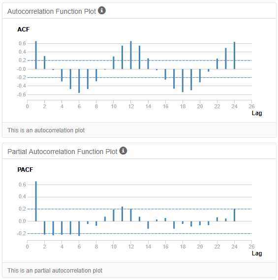
As explored previously, time series records have strong relationships with previous points in the data. The strength of these relationships can be measured through a statistical tool called autocorrelation.
An autocorrelation function (ACF) measures how much current data points in a time series are correlated to previous ones over different periods. It’s a method to understand how past values in the series influence current values.
Source: Alteryx
When generating synthetic data, it’s important to preserve these underlying patterns and correlations. Accurate synthetic datasets can mimic these patterns, successfully retaining both the statistical properties as well as the time-lagged behavior of the original time series.
Building predictive time series forecasts: ARIMA
Once the exploration of a time series is complete, analysts can use their findings to build predictive models against the dataset to forecast future values.
ARIMA, AutoRegressive Integrated Moving Average, is a popular statistical method effective for time series data showing patterns or trends over time. It combines three key components:
- Autoregression (AR): Using the relationship between a current observation and several lagged observations.
- Integration (I): A process to remove trends and seasonality from the data, effectively rendering it “stationary.”
- Moving Average (MA): Calculates the relationship between a current observation and the errors from previous predictions, helping to smooth out random noise in the data.
Building predictive time series forecasts: ETS
An alternative approach is to use a method known as Error, Trend, Seasonality (ETS) that focuses on decomposing a time series into its error, trend, and seasonal components to predict future values:
- Error: As seen in the decomposition plot above, the error component captures randomness or noise in the data.
- Trend: Captures the long-term progression in the time series.
- Seasonality: Captures any systematic or calendar-related patterns.
Reviewing forecasts: Visualization and statistics
Once a model (or models) have been created, they can be visualized alongside historical data to inspect how closely the forecast follows the pattern of the existing time series data.
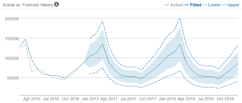
Source: phData
A quantitative approach to measuring time series forecasts often employs either the AIC (Akaike Information Criterion) or AICc (Corrected Akaike Information Criterion), defined as follows:
- AIC: Balances a model’s fit to the data against the complexity of the model, with a lower AIC score indicating a better model. AIC is often used when the sample size is significantly larger than the number of model parameters.
- AICc: This approach prevents overfitting in time series forecasting models with a smaller sample size by adding a correction term to the AIC calculation.
How to anonymize a time series with synthetic data
Anonymizing time series data is notoriously difficult and legacy anonymization approaches fail at this challenge.
But there is an effective alternative: synthetic data which offers a solution to these privacy concerns.
Synthesizing time series data makes a lot of sense when dealing with behavioral data. Understanding the key concepts of data subjects is a crucial step in learning how to generate synthetic data in a privacy-preserving manner.
A subject is an entity or individual whose privacy you will protect. Behavioral event data must be prepared in advance so that each subject in the dataset (e.g., a customer, website visitor, hospital patient, etc.) is stored in a dedicated table, each with a unique row identifier. These subjects can have additional reference information stored in separate columns, including attributes that ideally don’t change during the captured events.
For data practitioners, the concept of the subject table is similar to a “dimension” table in a data warehouse, where common attributes related to the subjects are provided for context and further analysis.
The behavioral event data is prepared and stored in a separate linked table referencing a unique subject. In this way, one subject will have zero, one, or (likely) many events captured in this linked table.
Records in the linked table must be pre-sorted in chronological order for each subject to capture the time-sensitive nature of the original data. This model suits various types of event-based data, including insurance claims, patient health, eCommerce, and financial transactions.
In the example of a customer journey, our tables may look like this.
We see customers stored in our subject table with their associated demographic attributes.
| ID | ZONE | STATE | GENDER | AGE_CAT | AGE |
|---|---|---|---|---|---|
| 1 | Pacific | Oregon | M | Young | 26 |
| 2 | Eastern | New Jersey | M | Medium | 36 |
| 3 | Central | Minnesota | M | Young | 17 |
| 4 | Eastern | Michigan | M | Medium | 56 |
| 5 | Eastern | New Jersey | M | Medium | 46 |
| 6 | Mountain | New Mexico | M | Medium | 35 |
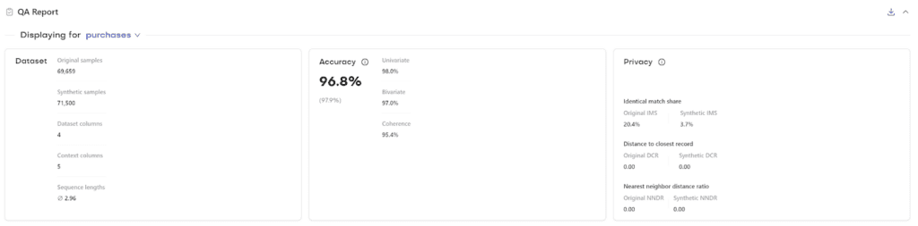
In the corresponding linked table, we have captured events relating to the purchasing behavior of each of our subjects.
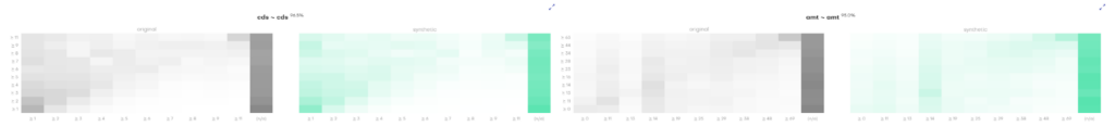
| USER_ID | DATE | NUM_CDS | AMT |
|---|---|---|---|
| 1 | 1997-01-01 | 1 | 11.77 |
| 2 | 1997-01-12 | 1 | 12 |
| 2 | 1997-01-12 | 5 | 77 |
In this example, user 1 visited the website on January 1st, 1997, purchasing 1 CD for $11.77. User 2 visited the website twice on January 12th, 1997, making six purchases over these visits for $89.
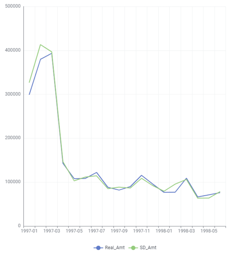
These consumer buying behaviors can be aggregated into standard metrics-based time series, such as purchases per week, month, or quarter, revealing general buying trends over time. Alternatively, the behavioral data in the linked table can be treated as discrete purchasing events happening at specific intervals in time.
Customer-centric organizations obsess around behaviors that drive revenue and retention beyond simple statistics. Analysts constantly ask questions about customer return rates, spending habits, and overall customer lifetime value.
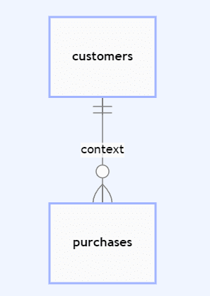
Synthetic data modeling: Relationships between subjects and linked data
Defining the relationship between customers and their purchases is an essential first step in synthetic data modeling. Ensuring that primary and foreign keys are identified between subject and linked tables enables synthetic data generation platforms to understand the context of each behavioral record (e.g., purchases) in terms of the subject (e.g., customers).
Additional configurations, such as smart imputation, dataset rebalancing, or rare category protection, can be defined at this stage.
Synthetic data modeling: Sequence lengths and continuation
A time series sequence refers to a captured set of data over time for a subject within the dataset. For synthetic data models, generating the next element in a sequence given a previous set of features is a critical capability known as sequence continuation.
Defining sequence lengths in synthetic data models involves specifying the number of time steps or data points to be considered in each sequence within the dataset. This decision determines how much historical data the synthetic model will use to predict or generate the next element in the sequence.
The choice of sequence length depends significantly on the nature of the data and the specific application. Longer sequence lengths can capture more long-term patterns and dependencies but will also require more computational resources and may need to be more responsive to recent changes. Conversely, a shorter sequence length is more sensitive to recent trends but might overlook longer-term patterns.
In synthetic modeling, selecting a sequence length that strikes a balance between capturing sufficient historical or behavioral context and maintaining computational efficiency and performance is essential.
Synthetic data generation: Accurate and privacy-safe results
Synthetic data generation can produce realistic and representative behavioral time series data that mimics the original distribution found in the source data without the possibility of re-identification. With privacy-safe behavioral data, it’s possible to democratize access to datasets such as these, developing more sophisticated behavioral models and deeper insights beyond basic metrics, “average” customers, and crude segmentation methods.