In this tutorial, you will learn how to perform conditional data generation. As the name suggests, this method of synthetic data generation is useful when you want to have more fine-grained control over the statistical distributions of your synthetic data by setting certain conditions in advance. This can be useful across a range of use cases, such as performing data simulation, tackling data drift, or when you want to retain certain columns as they are during synthesization.
You will work through two use cases in this tutorial. In the first use case, you will be working with the UCI Adult Income dataset in order to simulate what this dataset would look like if there was no gender income gap. In the second use case, you will be working with Airbnb accommodation data for Manhattan, which contains geolocation coordinates for each accommodation.
To gain useful insights from this dataset, this geolocation data will need to remain exactly as it is in the original dataset during synthesization. In both cases, you will end up with data that is partially pre-determined by the user (to either remain in its original form or follow a specific distribution) and partially synthesized.
It’s important to note that the synthetic data you generate using conditional data generation is still statistically representative within the conditional context that you’ve created. The degree of privacy preservation of the resulting synthetic dataset is largely dependent on the privacy of the provided fixed attributes.
The Python code for this tutorial is publicly available and runnable in this Google Colab notebook.
How does conditional data generation work?
We’ve broken down the process of conditional data generation with MOSTLY AI into 5 steps below. We’ll describe the steps here first, and in the following sections, you will get a chance to implement them yourself.
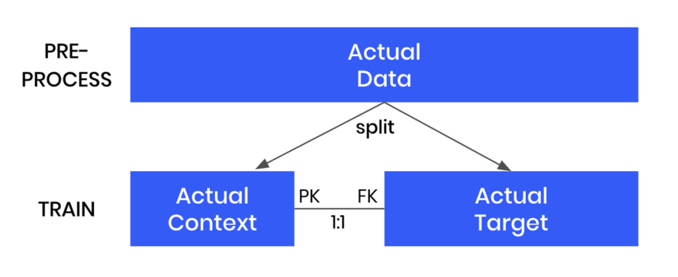
- We’ll start by splitting the original data table into two tables. The first table should contain all the columns that you want to hold fixed, the conditions based on which you want to generate your partially synthetic data. The second table will contain all the other columns, which will be synthesized within the context of the first table.
- We’ll then define the relationship between these two tables. The first table (containing the context data) should be set as a subject table, and the second table (containing the target data to be synthesized) as a linked table.
- Next, we will train a MOSTLY AI synthetic data generation model using this two-table setup. Note that this is just an intermediate step that will, in fact, create fully synthetic data since we are using the full original dataset (just split into two) and have not set any specific conditions yet.
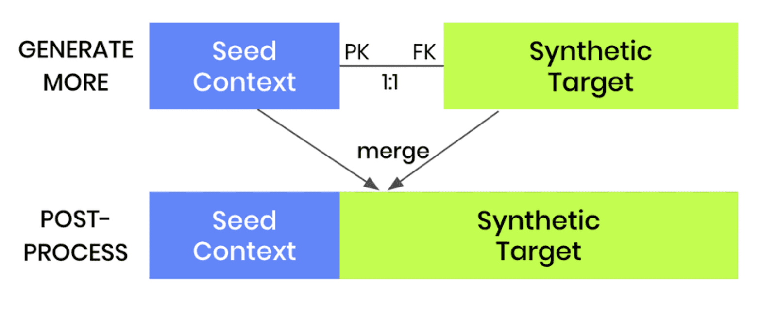
- Once the model is trained, we can then use it to generate more data by selecting the “Generate with seed” option. This option allows you to set conditions within which to create partially synthetic data. Any data you upload as the seed context will be used as fixed attributes that will appear as they are in the resulting synthetic dataset. Note that your seed context dataset must contain a matching ID column. The output of this step will be your synthetic target data.
- As a final post-processing step, we’ll merge the seed context with fixed attribute columns to your synthetic target data to get the complete, partially synthetic dataset created using conditional data generation.
Note that this same kind of conditional data generation can also be performed for two-table setups. The process is even easier in that case, as the pre-and post-processing steps are not required. Once a two-table model is trained, one can simply generate more data and provide a new subject table as the seed for the linked table.
Let’s see it in practice for our first use case: performing data simulation on the UCI Adult Income dataset to see what the data would look like if there was no gender income gap.
Conditional data generation for data simulation
For this use case, we will be using a subset of the UCI Adult Income dataset, consisting of 10k records and 10 attributes. Our aim here is to provide a specific distribution for the sex and income columns and see how the other columns will change based on these predetermined conditions.
Preprocess your data
As described in the steps above, your first task will be to enrich the dataset with a unique ID column and then split the data into two tables, i.e. two CSV files. The first table should contain the columns you want to control, in this case, the sex and income columns. The second table should contain the columns you want to synthesize, in this case, all the other columns.
df = pd.read_csv(f'{repo}/census.csv')
# define list of columns, on which we want to condition on
ctx_cols = ['sex', 'income']
tgt_cols = [c for c in df.columns if c not in ctx_cols]
# insert unique ID column
df.insert(0, 'id', pd.Series(range(df.shape[0])))
# persist actual context, that will be used as subject table
df_ctx = df[['id'] + ctx_cols]
df_ctx.to_csv('census-context.csv', index=False)
display(df_ctx.head())
# persist actual target, that will be used as linked table
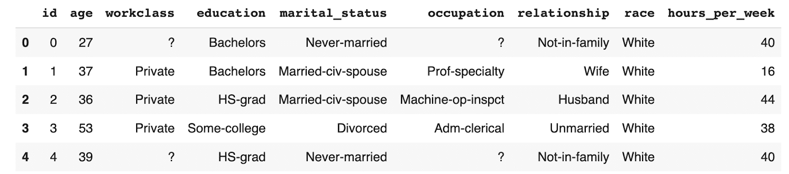
df_tgt = df[['id'] + tgt_cols]
df_tgt.to_csv('census-target.csv', index=False)
display(df_tgt.head())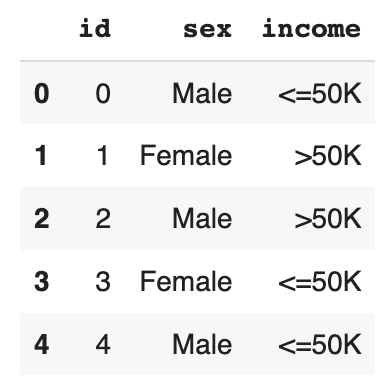
Save the resulting tables to disk as CSV files in order to upload them to MOSTLY AI in the next step. If you are working in Colab this will require an extra step (provided in the notebook) in order to download the files from the Colab server to disk.
Train a generative model with MOSTLY AI
Use the CSV files you have just created to train a synthetic data generation model using MOSTLY AI.
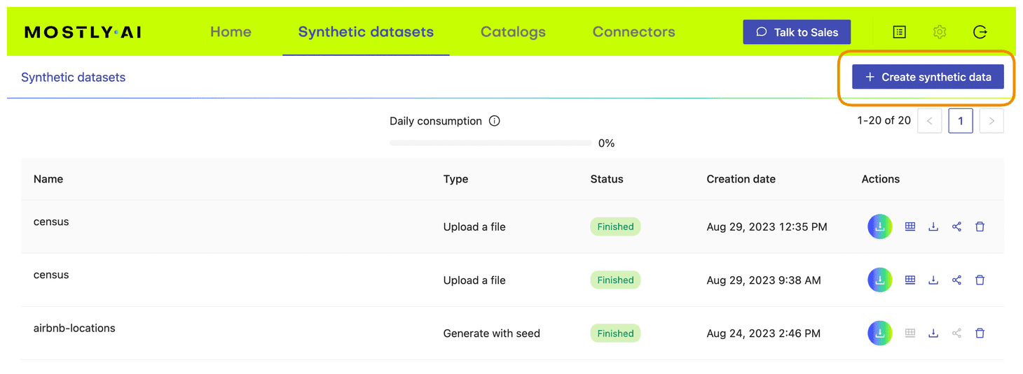
- Navigate to your MOSTLY AI account and go to the “Synthetic datasets” tab. Click on “Create synthetic data” to start a new job.
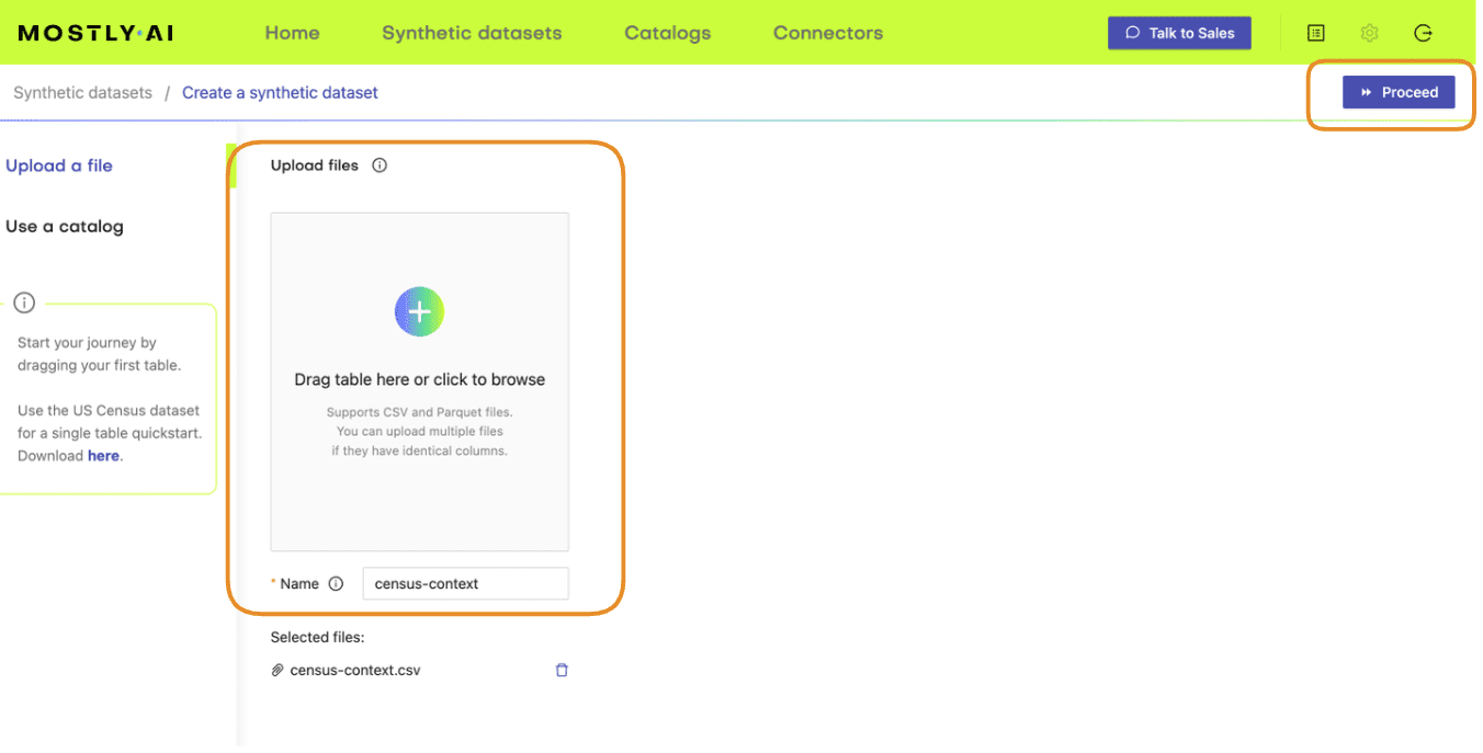
- Upload the census-context.csv (the file containing your context data).
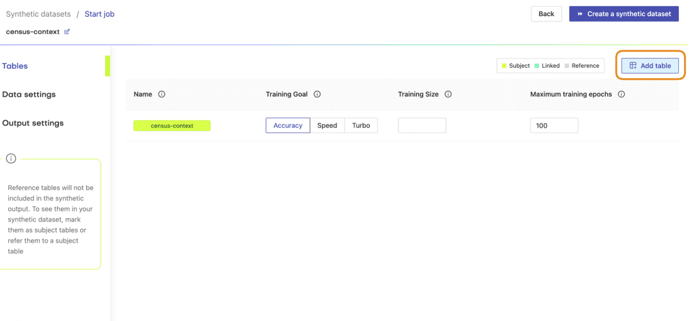
- Once the upload is complete, click on “Add table” and upload census-target.csv (the file containing your target data) here.
- Next, define the table relationship by navigating to “Data Settings,” selecting the ID column of the context table, and setting the following settings:
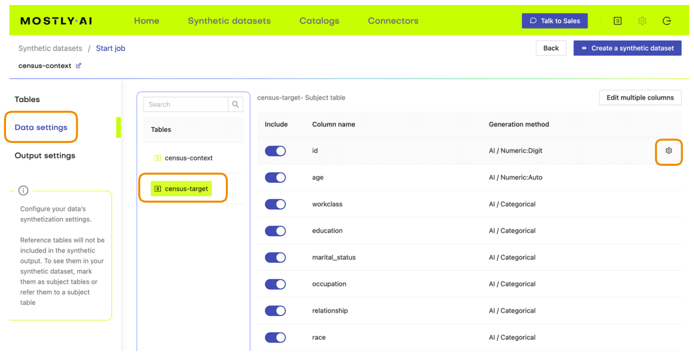
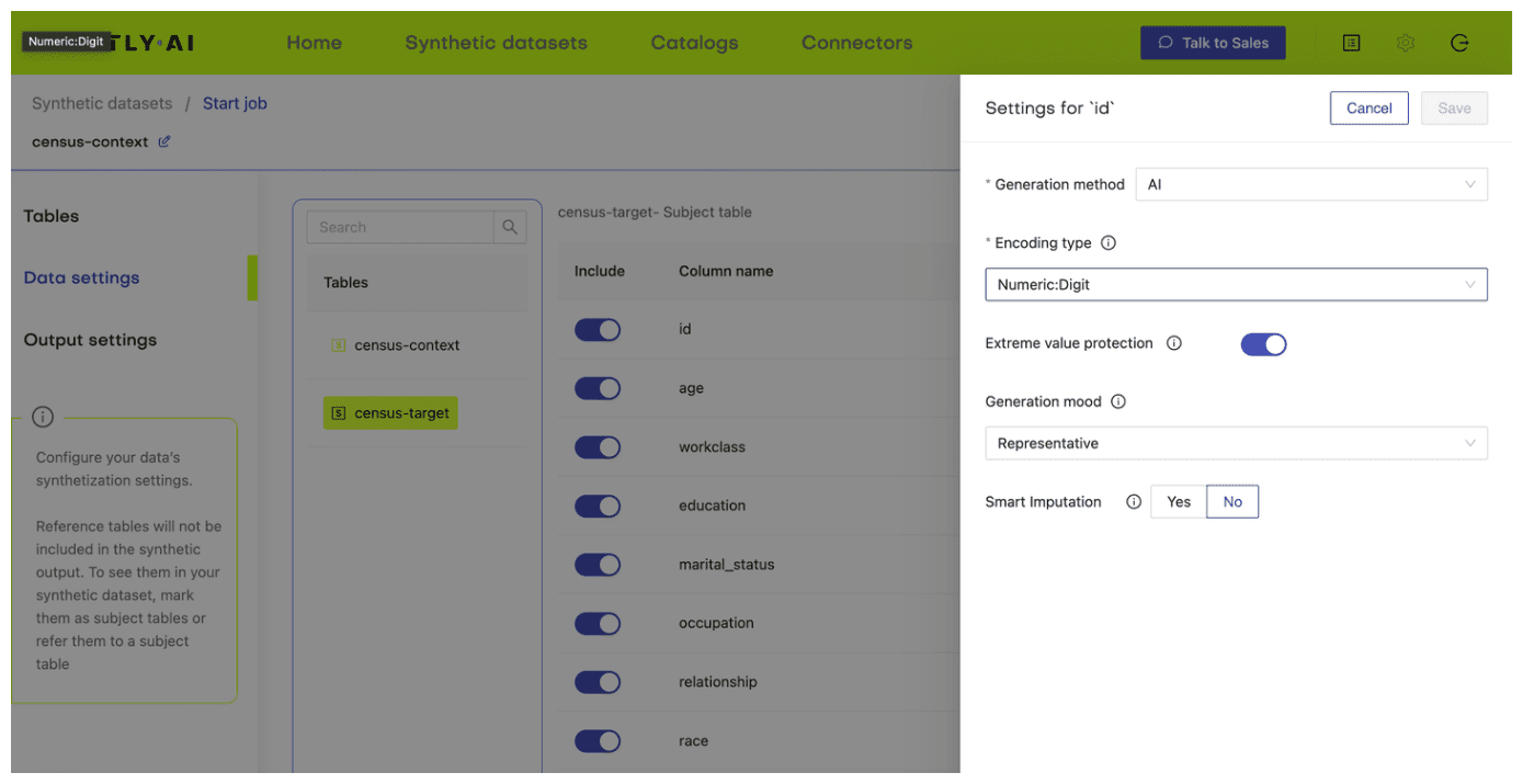
- Confirm that your census-context table is now set as the subject table and the
census-targetas linked table.
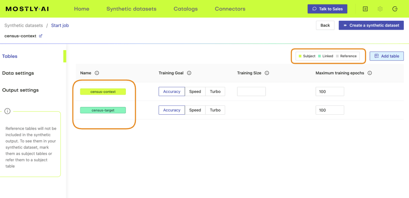
- Click “Create a synthetic dataset” to launch the job and train the model. As noted before, the resulting synthetic data is not of particular interest at the moment. We are interested in the model that is created and will use it for conditional data generation in the next section.
Conditional data generation with MOSTLY AI
Now that we have our base model, we will need to specify the conditions within which we want to create synthetic data. For this first use case, you will simulate what the dataset will look like if there was no gender income gap.
- Create a CSV file that contains the same columns as the context file but now containing the specific distributions of those variables you are interested in simulating. In this case, we’ll create a dataset containing an even split between male and female records as well as an even distribution of high- and low-income records. You can use the code block below to do this.
import numpy as np
np.random.seed(1)


n = 10_000
p_inc = (df.income=='>50K').mean()
seed = pd.DataFrame({
    'id': [f's{i:04}' for i in range(n)],
    'sex': np.random.choice(['Male', 'Female'], n, p=[.5, .5]),
    'income': np.random.choice(['<=50K', '>50K'], n, p=[1-p_inc, p_inc]),
})
seed.to_csv('census-seed.csv', index=False)
seed.sample(8)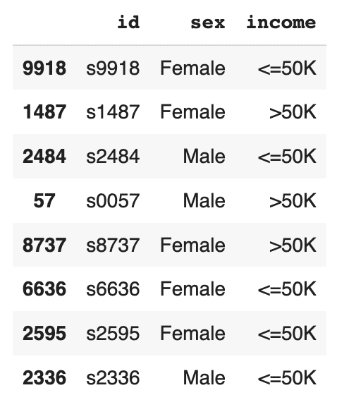
The resulting DataFrame contains an even income split between males and females, i.e. no gender income gap.
- Download this CSV to disk as
census-seed.csv
- In your MOSTLY AI account, click on the “Generate more data” button located to the right of the model that you have just trained.
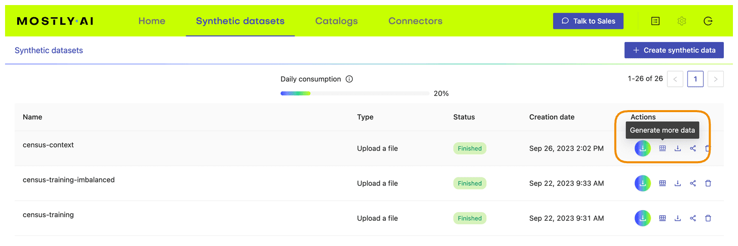
- Select the “Generate with seed” option. This allows you to specify conditions that the synthesization should respect. Upload
census-seed.csvhere.
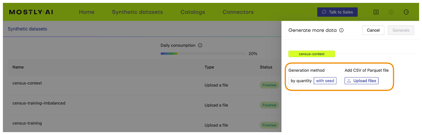
- Generate more data by clicking on “Generate”. Once completed, download the resulting synthetic dataset as CSV.
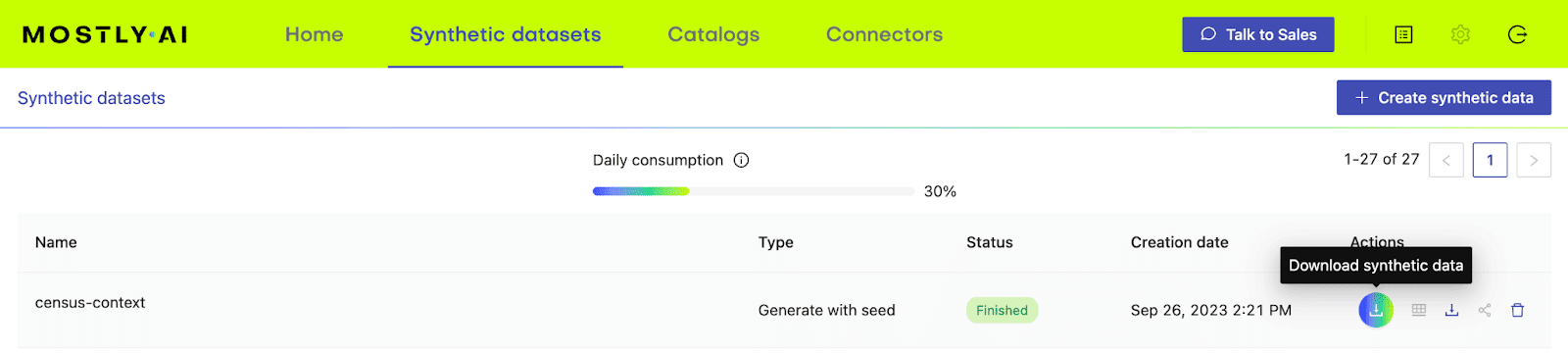
- Merge the synthetic target data to your seed context columns to get your complete, conditionally generated dataset.
# merge fixed seed with synthetic target to
# a single partially synthetic dataset
syn = pd.read_csv(syn_file_path)
syn = pd.merge(seed, syn, on='id').drop(columns='id')
Explore synthetic data
Let’s take a look at the data you have just created using conditional data generation. Start by showing 10 randomly sampled synthetic records. You can run this line multiple times to see different samples.
syn.sample(n=10)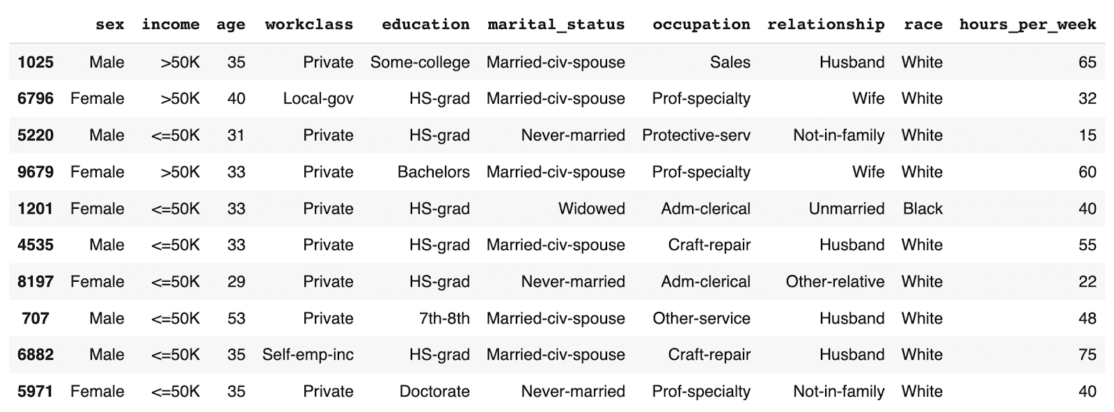
You can see that the partially synthetic dataset consists of about half male and half female records.
Let's now compare the age distribution of records from the original data against those from the partially synthetic data. We’ll plot both the original and synthetic distributions on a single plot to compare.
import matplotlib.pyplot as plt
plt.xlim(10, 95)
plt.title('Female Age Distribution')
plt.xlabel('Age')
df[df.sex=='Female'].age.plot.kde(color='black', bw_method=0.2)
syn[syn.sex=='Female'].age.plot.kde(color='#24db96', bw_method=0.2)
plt.legend({'original': 'black', 'synthetic': '#24db96'})
plt.show()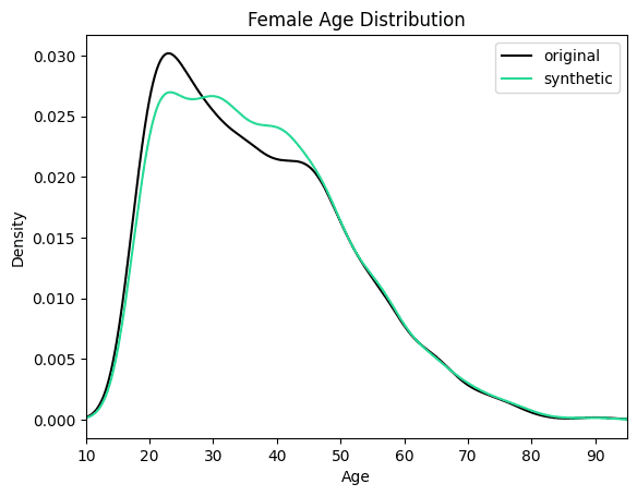
We can see clearly that the synthesized female records are now significantly older in order to meet the criteria of removing the gender income gap. Similarly, you can now study other shifts in the distributions that follow as a consequence of the provided seed data.
Conditional generation to retain original data
In the above use case, you customized your data generation process in order to simulate a particular, predetermined distribution for specific columns of interest (i.e. no gender income gap). In the following section, we will explore another useful application of conditional generation: retaining certain columns of the original dataset exactly as they are while letting the rest of the columns be synthesized. This can be a useful tool in situations when it is crucial to retain parts of the original dataset.
In this section, you will be working with a dataset containing the 2019 Airbnb listings in Manhattan. For this use case, it is crucial to preserve the exact locations of the listings in order to avoid situations in which the synthetic dataset contains records in impossible or irrelevant locations (in the middle of the Hudson River, for example, or outside of Manhattan entirely).
You need the ability to execute control over the location column to ensure the relevance and utility of your resulting synthetic dataset - and conditional data generation gives you exactly that level of control.
Let’s look at this type of conditional data generation in action. Since many of the steps will be the same as in the use case above, this section will be a bit more compact.
Preprocess your data
Start by enriching the DataFrame with an id column. Then split it into two DataFrames: airbnb-context.csv and airbnb-target.csv. Additionally, you will need to concatenate the latitude and longitude columns together into a single column. This is the format expected by MOSTLY AI, in order to improve its representation of geographical information.
df_orig = pd.read_csv(f'{repo}/airbnb.csv')

df = df_orig.copy()

# concatenate latitude and longitude to "LAT, LONG" format
df['LAT_LONG'] = (
    df['latitude'].astype(str) + ', ' + df['longitude'].astype(str)
)
df = df.drop(columns=['latitude', 'longitude'])

# define list of columns, on which we want to condition on
ctx_cols = ['neighbourhood', 'LAT_LONG']
tgt_cols = [c for c in df.columns if c not in ctx_cols]

# enricht with ID column
df.insert(0, 'id', pd.Series(range(df.shape[0])))

# persist actual context, that will be used as subject table
df_ctx = df[['id'] + ctx_cols]
df_ctx.to_csv('airbnb-locations.csv', index=False)
display(df_ctx.head())

# persist actual target, that will be used as linked table
df_tgt = df[['id'] + tgt_cols]
df_tgt.to_csv('airbnb-data.csv', index=False)
display(df_tgt.head())
Train generative model with MOSTLY AI
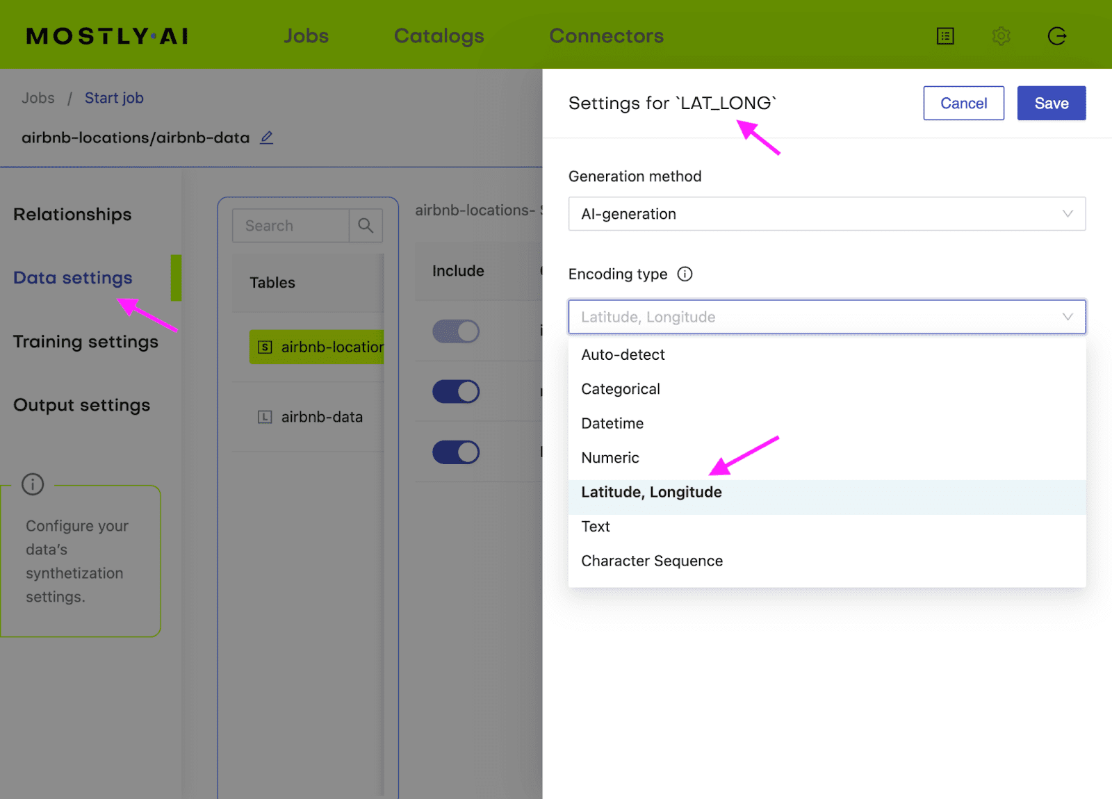
Follow the same steps as in the first use case to train a generative model with MOSTLY AI. Upload airbnb-locations.csv first, then add the airbnb-data.csv file and define the table relationship by setting the ID column of the airbnb-data table as the Foreign Key pointing to the ID column of the airbnb-locations file. Refer to the detailed steps in the first use case if you need a refresher on how to do that.
Additionally, you will need to configure the LAT_LONG column to the encoding type Lat, Long in order for MOSTLY AI to correctly process this geolocation data.
Generate more data with MOSTLY AI
Once the training has finished, you can generate your partially synthetic data. In the previous example, this is where we uploaded the seed context file that we generated. In this case, we actually want our fixed attributes to remain exactly as they are in the original dataset. This means you can simply re-upload the original airbnb-locations.csv as the seed file to the "generate more data" form. Once the data has been generated, download the data as a CSV file again. Merge the two files (seed and synthetic target) and split the LAT_LONG column back into separate latitude and longitude columns.
# merge fixed seed with synthetic target
# to a single partially synthetic dataset
syn = pd.read_csv(syn_file_path)
syn_partial = pd.merge(df_ctx, syn, on='id')

# split LAT_LONG into separate columns again
syn_partial = pd.concat([
    syn_partial,
    syn_partial.LAT_LONG.str.split(', ', n=2, expand=True).rename(columns={0: 'latitude', 1: 'longitude'}).astype(float),
], axis=1).drop(columns='LAT_LONG')

# restore column order
syn_partial = syn_partial[df_orig.columns]
Explore synthetic data
Let's compare the price distribution of listings across Manhattan. Note that while the locations in the partially synthetic data are actual locations, all other attributes, including the price per night, are randomly sampled by the generative model. Still, these prices remain statistically representative given the context, i.e. the location within Manhattan.
The code block below plots the price distribution of the original dataset as well as that of the partially synthetic dataset. We hope to see the exact same locations (so no listings in the middle of the Hudson River) and a price distribution that is statistically similar but not exactly the same.
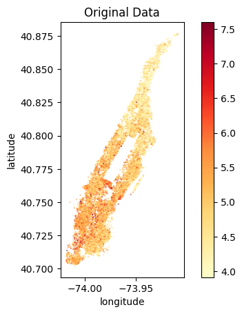
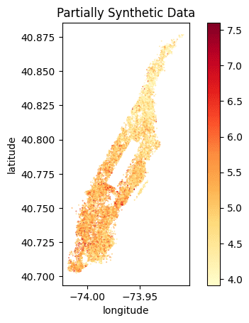
We can clearly see that the locations of the listings have been preserved and the price distribution is accurately represented. We can see a similar gradient of lower prices per night in the Northern tip of Manhattan as well as high prices per night at the Southern end of Central Park and the Financial District.
Of course, you could also create fully synthetic data for this use case, and this will yield statistically representative locations with their attributes. However, as these locations do not necessarily exist (e.g. they might end up in the Hudson River), the demonstrated approach allows you to combine the best of both worlds.
Conditional data generation with MOSTLY AI
In this tutorial, you have learned how to perform conditional data generation. You have explored the value conditional generation can provide by working through two use cases: one in which you simulated a specific distribution for a subset of the columns (the Adult Income dataset with no gender income gap) and another in which you retained certain columns of the original dataset (the locations of the Airbnb listings). In both cases, you were able to execute more fine-grained control over the statistical distributions of your synthetic data by setting certain conditions in advance.
The result is a dataset that is partially pre-determined by the user (to either remain in its original form or follow a specific distribution) and partially synthesized. You can now put your conditional data generation skill to use for data simulation, to tackle data drift, or for other relevant use cases.
What’s next?
In addition to walking through the above instructions, we suggest experimenting with the following to get an even deeper understanding of conditional data generation:
- use a different set of fixed columns for the US Census dataset
- generate a very large number of records for a fixed value set, e.g. create 1 million records of 48-year-old female Professors
- perform a fully synthetic dataset of the Airbnb Manhattan dataset
Synthetic data holds the promise of addressing the underrepresentation of minority classes in tabular data sets by adding new, diverse, and highly realistic synthetic samples. In this post, we'll benchmark AI-generated synthetic data for upsampling highly unbalanced tabular data sets. Specifically, we compare the performance of predictive models trained on data sets upsampled with synthetic records to that of well-known upsampling methods, such as naive oversampling or SMOTE-NC.
Our experiments are conducted on multiple data sets and different predictive models. We demonstrate that synthetic data can improve predictive accuracy for minority groups as it creates diverse data points that fill gaps in sparse regions in feature space.
Our results highlight the potential of synthetic data upsampling as a viable method for improving predictive accuracy on highly unbalanced data sets. We show that upsampled synthetic training data consistently results in top-performing predictive models, in particular for mixed-type data sets containing a very low number of minority samples, where it outperforms all other upsampling techniques.
Try upsampling on MOSTLY AI's synthetic data platform!
The definition of synthetic data
AI-generated synthetic data, which we refer to as synthetic data throughout, is created by training a generative model on the original data set. In the inference phase, the generative model creates statistically representative, synthetic records from scratch.
The use of synthetic data has gained increasing importance in various industries, particularly due to its primary use case of enhancing data privacy. Beyond privacy, synthetic data offers the possibility to modify and tailor data sets to our specific needs. In this blog post, we investigate the potential of synthetic data to improve the performance of machine learning algorithms on data sets with unbalanced class distributions, specifically through the synthetic upsampling of minority classes.
Upsampling for class imbalance
Class imbalance is a common problem in many real-world tabular data sets where the number of samples in one or more classes is significantly lower than the others. Such imbalances can lead to poor prediction performance for the minority classes, often of greatest interest in many applications, such as detecting fraud or extreme insurance claims.
Traditional upsampling methods, such as naive oversampling or SMOTE, have shown some success in mitigating this issue. However, the effectiveness of these methods is often limited, and they may introduce biases in the data, leading to poor model performance. In recent years, synthetic data has emerged as a promising alternative to traditional upsampling methods. By creating highly realistic samples for minority classes, synthetic data can significantly improve the accuracy of predictive models.
While upsampling methods like naive oversampling and SMOTE are effective in addressing unbalanced data sets, they also have their limitations. Naive oversampling mitigates class imbalance effects by simply duplicating minority class examples. Due to this strategy, they bear the risk of overfitting the model to the training data, resulting in poor generalization in the inference phase.
SMOTE, on the other hand, generates new records by interpolating between existing minority-class samples, leading to higher diversity. However, SMOTE’s ability to increase diversity is limited when the absolute number of minority records is very low. This is especially true when generating samples for mixed-type data sets containing categorical columns. For mixed-type data sets, SMOTE-NC is commonly used as an extension for handling categorical columns.
SMOTE-NC may not work well with non-linear decision boundaries, as it only linearly interpolates between minority records. This can lead to SMOTE-NC examples being generated in an “unfavorable” region of feature space, far from where additional samples would help the predictive model place a decision boundary.
All these limitations highlight the need for exploring alternative upsampling methods, such as synthetic data upsampling, that can overcome these challenges and improve the accuracy of minority group predictions.
The strength of upsampling minority classes with AI-generated synthetic data is that the generative model is not limited to upsampling or interpolating between existing minority classes. Most AI-based generators can create realistic synthetic data examples in any region of feature space and, thus, considerably increase diversity. Because they are not tied to existing minority samples, AI-based generators can also leverage and learn from the properties of (parts of) the majority samples that are transferable to minority examples.
An additional strength of using AI-based upsampling is that it can be easily extended to more complex data structures, such as sequential data, where not only one but many rows in a data set belong to a single data subject. This aspect of synthetic data upsampling is, however, out of the scope of this study.
In this post, we present a comprehensive benchmark study comparing the performance of predictive models trained on unbalanced data upsampled with AI-generated synthetic data, naive upsampling, and SMOTE-NC upsampling. Our experiments are carried out on various data sets and using different predictive models.
The upsampling experiment
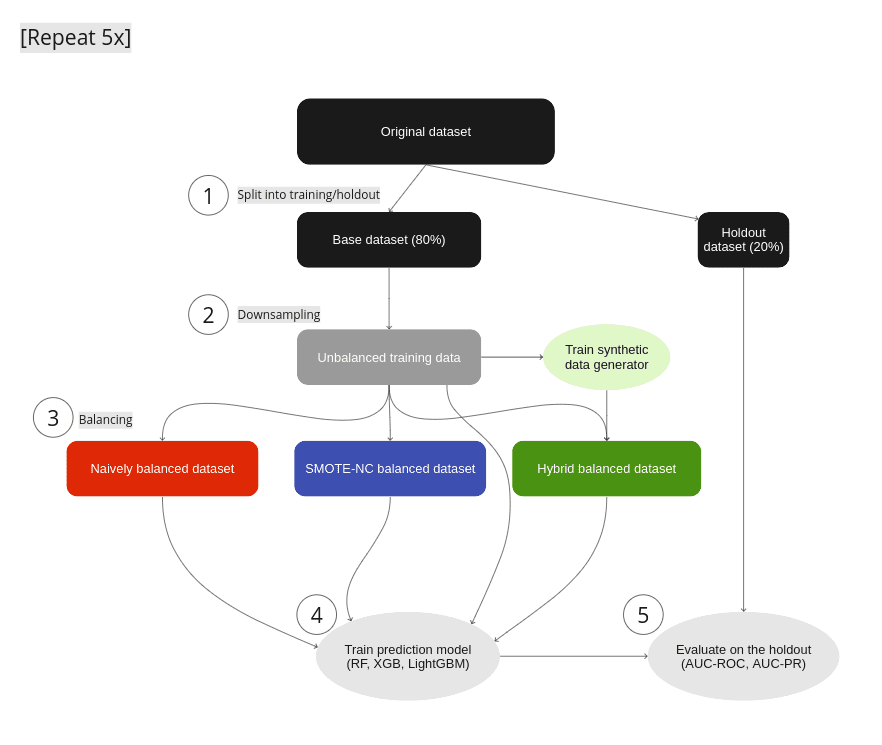
Figure 1: Experimental Setup: (1) We split the original data set into a base data set and a holdout. (2) Strong imbalances are introduced in the base data set by downsampling the minority classes to fractions as low as 0.05% to yield the unbalanced training data. (3) We test different mitigation strategies: balancing through naive upsampling, SMOTE-NC upsampling, and upsampling with AI-generated synthetic records (the hybrid data set). (4) We train LGBM, RandomForest, and XGB classifiers on the balanced and unbalanced training data. (5) We evaluate the properties of the upsampling techniques by measuring the performance of the trained classifier on the holdout set. Steps 1–5 are repeated five times, and we report the mean AUC-ROC as well as the AUC-PR.
For every data set we use in our experiments, we run through the following steps (see Fig. 1):
- We split the original data set into a base and a holdout set by using a five-fold stratified sampling approach to ensure that each class is represented proportionally.
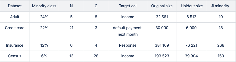
- All of the original data sets have a binary target column and only a rather moderate imbalance with the fraction of the minority class ranging from 6% to 24% (see table 1 for data set details). We artificially induce different levels of strong imbalances to the base set by randomly down-sampling the minority class, resulting in unbalanced training data sets with minority fractions of 0.05%, 0.1%, 0.2%, 0.5%, 1%, 2%, and 5%.
- To mitigate the strong imbalances in the training data sets, we apply three different upsampling techniques:
- naive oversampling (red box in fig. 1) duplicating existing examples of the minority classes (scikit-learn, RandomOverSampler)
- SMOTE-NC (blue box in fig. 1): applying the SMOTE-NC upsampling technique (scikit-learn, SMOTENC)
- Hybrid (green box in fig. 1): The hybrid data set represents the concept of enriching unbalanced training data with AI-generated synthetic data. It is composed of the training data (including majority samples and a limited number of minority samples) along with additional synthetic minority samples that are created using an AI-based synthetic data generator. This generator is trained on the highly unbalanced training data set. In this study, we use the MOSTLY AI synthetic data platform. It is freely accessible for generating highly realistic AI-based synthetic data.
In all cases, we upsample the minority class to achieve a 50:50 balance between the majority and minority classes, resulting in the naively balanced, the SMOTE-NC balanced, and the balanced hybrid data set.
- We assess the benefits of the different upsampling techniques by training three popular classifiers: RandomForest, XGB, and LightGBM, on the balanced data sets. Additionally, we train the classifiers on the heavily unbalanced training data sets as a baseline in the evaluation of the predictive model performance.
- The classifiers are scored on the holdout set, and we calculate the AUC-ROC score and AUC-PR score across all upsampling techniques and initial imbalance ratios for all 5 folds. We report the average scores over five different samplings and model predictions. We opt for AUC metrics to eliminate dependencies on thresholds, as seen in, e.g., F1 scores.
The results of upsampling
We run four publicly available data sets (Figure 1) of varying sizes through steps 1–5: Adult, Credit Card, Insurance, and Census (Kohavi and Becker). All data sets tested are of mixed type (categorical and numerical features) with a binary, that is, a categorical target column.
In step 2 (Fig. 1), we downsample minority classes to induce strong imbalances. For the smaller data sets with ~30k records, downsampling to minority-class fractions of 0.1% results in extremely low numbers of minority records.
The downsampled Adult and Credit Card unbalanced training data sets contain as little as 19 and 18 minority records, respectively. This scenario mimics situations where data is limited and extreme cases occur rarely. Such setups create significant challenges for predictive models, as they may encounter difficulty making accurate predictions and generalizing well on unseen data.
Please note that the holdout sets on which the trained predictive models are scored are not subject to extreme imbalances as they are sampled from the original data before downsampling is applied. The imbalance ratios of the holdout set are moderate and vary from 6 to 24%.
In the evaluation, we report both the AUC-ROC and the AUC-PR due to the moderate but inhomogeneous distribution of minority fractions in the holdout set. The AUC-ROC is a very popular and expressive metric, but it is known to be overly optimistic on unbalanced optimization problems. While the AUC-ROC considers both classes, making it susceptible to neglecting the minority class, the AUC-PR focuses on the minority class as it is built up by precision and recall.
Upsampling the Adult income dataset
The largest differences between upsampling techniques are observed in the AUC-ROC when balancing training sets with a substantial class imbalance of 0.05% to 0.5%. This scenario involves a very limited number of minority samples, down to 19 for the Adult unbalanced training data set.
For the RF and the LGBM classifiers trained on the balanced hybrid data set, the AUC-ROC is larger than the ones obtained with other upsampling techniques. Differences can go up to 0.2 (RF classifier, minority fraction of 0.05%) between the AI-based synthetic upsampling and the second-best method.
The AUC-PR shows similar yet less pronounced differences. LGBM and XGB classifiers trained on the balanced hybrid data set perform best throughout almost all minority fractions. Interestingly, results for the RF classifier are mixed. Upsampling with synthetic data does not always lead to better performance, but it is always among the best-performing methods.
While synthetic data upsampling improves results through most of the minority fractions for the XGB classifier, too, the differences in performance are less pronounced. Especially the XGB classifier trained on the highly unbalanced training data performs surprisingly well. This suggests that the XGB classifier is better suited for handling unbalanced data.
The reason for the performance differences in the AUC-ROC and AUC-PR is due to the low diversity and, consequently, overfitting when using naive or SMOTE-NC upsampling. These effects are visible in, e.g., the ROC and PR curves of the LGBM classifier for a minority fraction of 0.1% (fig. 3).
Every point on these curves corresponds to a specific prediction threshold for the classifier. The set of threshold values is defined by the variance of probabilities predicted by the models when scored on the holdout set. For both the highly unbalanced training data and the naively upsampled one, we observe very low diversity, with more than 80% of the holdout samples predicted to have an identical, very low probability of belonging to the minority class.
In the plot of the PR curve, this leads to an accumulation of points in the area with high precision and low recall, which means that the model is very conservative in making positive predictions and only makes a positive prediction when it is very confident that the data point belongs to the positive, that is, the minority class. This demonstrates the effect of overfitting on a few samples in the minority group.
SMOTE-NC has a much higher but still limited diversity, resulting in a smoother PR curve which, however, still contains discontinuities and has a large segment where precision and recall change rapidly with small changes in the prediction threshold.
The hybrid data set offers high diversity during model training, resulting in almost every holdout sample being assigned an unique probability of belonging to the minority class. Both ROC and PR curves are smooth and have a threshold of ~0.5 at the center, the point that is closest to the perfect classifier.
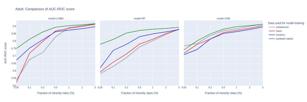
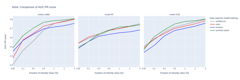
Figure 2: AUC-ROC (top) and AUC-PR (bottom) of classifiers LGBM, RandomForest (RF), and XGB trained on the Adult data set to predict the target feature income. The classifiers are trained on unbalanced data sets (grey) and data sets that are upsampled naively (red), with the SMOTE-NC algorithm (blue), and with AI-generated synthetic records (green). AUC values are reported for different fractions of the minority class in the unbalanced training data (x-axis).
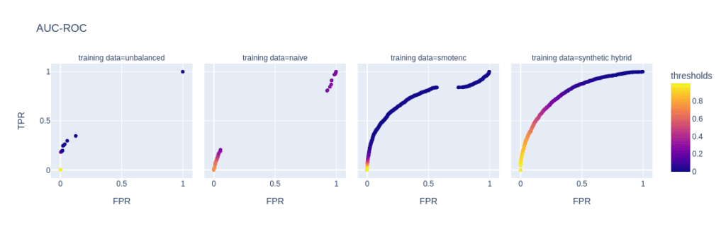
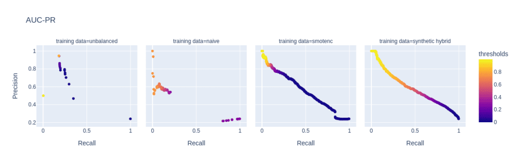
Figure 3: ROC (top) and PR (bottom) curves of the Light GBM classifier trained on different versions of the adult data set (from left to right): unbalanced training data (minority class fraction 0.1%), naively upsampled training data, training data upsampled with SMOTE-NC, and training data enriched with AI-generated synthetic records (synthetic hybrid). Every point on the plots corresponds to a specific prediction threshold for the classifier.
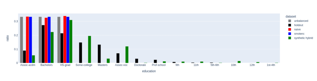
Figure 4: Distribution of the feature education for the female subgroup (sex equals female) of the minority class (income equals high). The distributions of the unbalanced (grey, minority class fraction of 0.1%), the naively upsampled (red), and the SMOTE-NC upsampled (blue) considerably differ from the holdout distribution. Only the data set upsampled with AI-generated synthetic records (synthetic hybrid) recovers the holdout distribution to a satisfactory degree and captures its diversity.
The limited power in creating diverse samples in situations where the minority class is severely underrepresented stems from naive upsampling and SMOTE-NC being limited to duplicating and interpolating between existing minority samples. Both methods are bound to a limited region in feature space.
Upsampling with AI-based synthetic minority samples, on the other hand, can, in principle, populate any region in feature space and can leverage and learn from properties of the majority samples which are transferable to minority examples, resulting in more diverse and realistic synthetic minority samples.
We analyze the difference in diversity by further “drilling down” the minority class (feature “income” equals “high”) and comparing the distribution of the feature “education” for the female subgroup (feature “sex” equals “female”) in the upsampled data sets (fig. 4).
For a minority fraction of 0.1%, this results in only three female minority records. Naive upsampling and SMOTE-NC have a very hard time generating diversity in such settings. Both just duplicate the existing categories “Bachelors”, “HS-grade”, and "Assoc-acdm,” resulting in a strong distortion of the distribution of the “education” feature as compared to the distribution in the holdout data set.
The distribution of the hybrid data has some imperfections, too, but it recovers the holdout distribution to a much better degree. Many more “education” categories are populated, and, with a few exceptions, the frequencies of the holdout data set are recovered to a satisfactory level. This ultimately leads to a larger diversity in the hybrid data set than in the naively balanced or SMOTE-NC balanced one.
Diversity assessment with the Shannon entropy
We quantitatively assess diversity with the Shannon entropy, which measures the variability within a data set particularly for categorical data. It provides a measure of how uniformly the different categories of a specific feature are distributed within the data set.
The Shannon Entropy (SE) of a specific feature is defined as
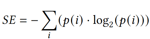
where p(i) represents the probability of occurrence, i.e. the relative frequency of category i. SE ranges from 0 to log2(N), where N is the total number of categories. A value of 0 indicates maximum certainty with only one category, while higher entropy implies greater diversity and uncertainty, indicating comparable probabilities p(i) across categories.
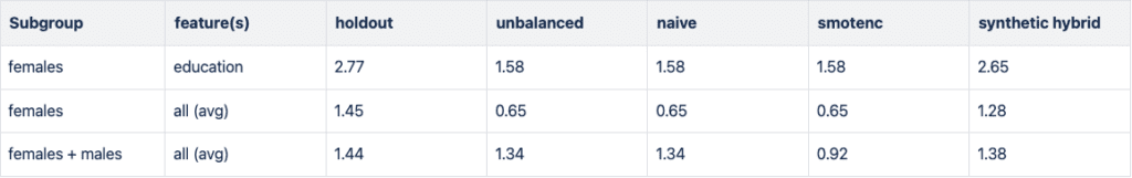
In Figure 5, we report the Shannon entropy for different features and subgroups of the high-income population. In all cases, data diversity is the largest for the holdout data set. The downsampled training data set (unbalanced) has a strongly reduced SE, especially when focusing on the small group of high-income women. Naive and SMOTE-NC upsampling cannot recover any of the diversity in the holdout as both are limited to the categories present in the minority class. In line with the results presented in the paragraph above, synthetic data recovers the SE, i.e., the diversity of the holdout data set, to a large degree.
Upsampling the Credit Card data set
The Credit Card data set has similar properties as the Adult data set. The number of records, features, and the original, moderate imbalance are comparable. This again results in a very small number of minority records (18) after downsampling to a 0.1% minority fraction.
The main difference between them is the fact that Credit Card consists of more numeric features. The performance of different upsampling techniques on the unbalanced Credit Card training data set shows similar results to the Adult Data set, too. AUC-ROC and AUC-PR for both LGBM and RF classifiers improve over naive upsampling and SMOTE-NC when using the hybrid data set.
Again, the performance of the XGB model is more comparable between the different balanced data sets and we find very good performance for the highly-unbalanced training data set. Here, too, the hybrid data set is always among the best-performing upsampling techniques.
Interestingly, SMOTE-NC performs worst almost throughout all the metrics. This is surprising because we expect this data set, consisting mainly of numerical features, to be favorable for the SMOTE-NC upsampling technique.
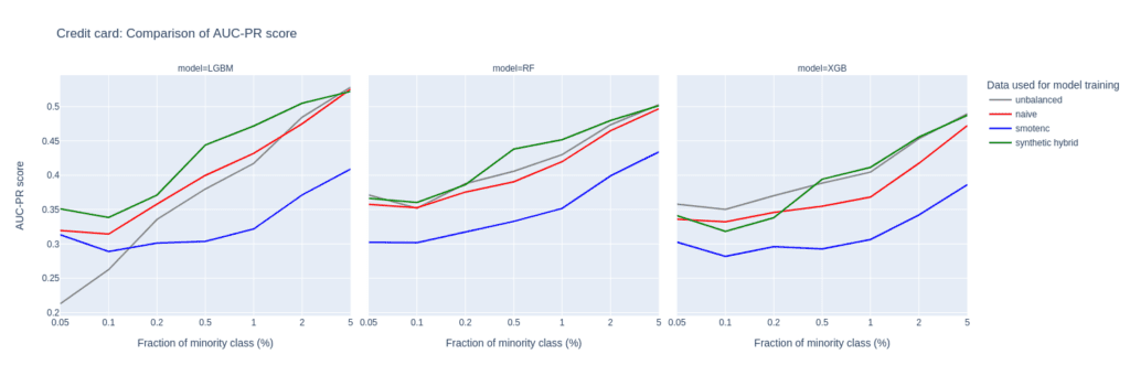
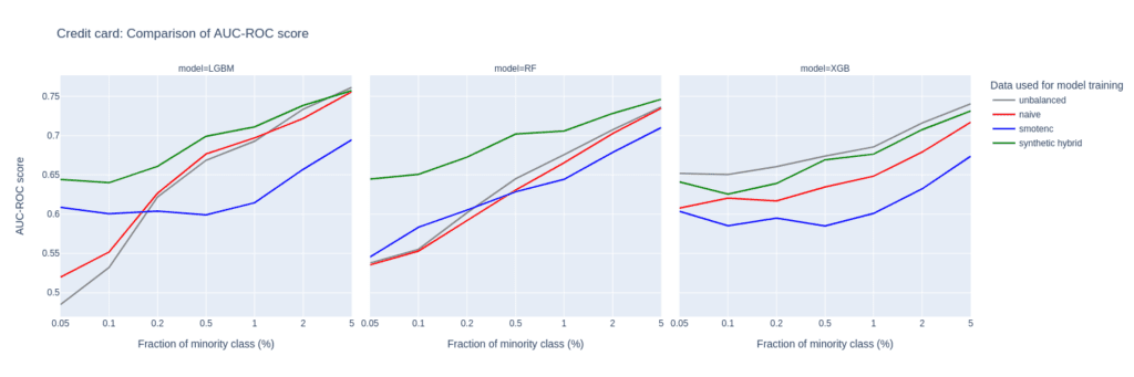
Figure 6: AUC-ROC (top) and AUC-PR (bottom) of classifiers LGBM, RandomForest (RF), and XGB trained on the Credit Card data set to predict the target feature default payment. The classifiers are trained on unbalanced data sets (grey) and data sets that are upsampled naively (red), with the SMOTE-NC algorithm (blue), and with AI-generated synthetic records (green). AUC values are reported for different fractions of the minority class in the unbalanced training data (x-axis).
Upsampling the Insurance data set
The Insurance data set is larger than Adult and Census resulting in a larger number of minority records (268) when downsampling to the 0.1% minority fraction. This leads to a much more balanced performance between different upsampling techniques.
A notable difference in performance only appears for very small minority fractions. For minority fractions below 0.5%, both the AUC-ROC and AUC-PR of LGBM and XGB classifiers trained on the hybrid data set are consistently larger than for classifiers trained on other balanced data sets. The maximum performance gains, however, are smaller than those observed for “Adult” and “Credit Card”.
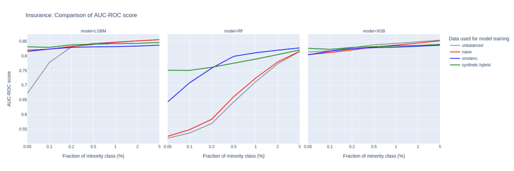
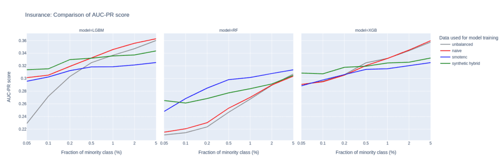
Figure 7: AUC-ROC (top) and AUC-PR (bottom) of classifiers LGBM, RandomForest (RF), and XGB trained on the Insurance data set to predict the target feature Response. The classifiers are trained on unbalanced data sets (grey) and data sets that are upsampled naively (red), with the SMOTE-NC algorithm (blue), and with AI-generated synthetic records (green). AUC values are reported for different fractions of the minority class in the unbalanced training data (x-axis).
Upsampling the Census data set
The Census data set has the largest number of features of all the data sets tested in this study. Especially, the 28 categorical features pose a challenge for SMOTE-NC, leading to poor performance in terms of AUC-PR.
Comparably to the Insurance data set, the performance of the LGBM classifier severely deteriorates when trained on highly unbalanced data sets. On the other hand, the XGB model excels and performs very well even on unbalanced training sets.
The Census data set highlights the importance of carefully selecting the appropriate model and upsampling technique when working with data sets that have high dimensionality and unbalanced class distributions, as performances can vary a lot.
Upsampling with synthetic data mitigates this variance, as all models trained on the hybrid data set are among the best performers across all classifiers and ranges of minority fractions.
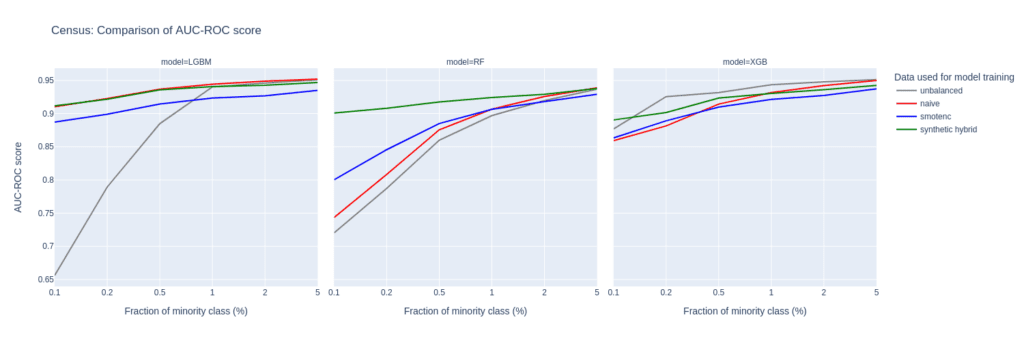
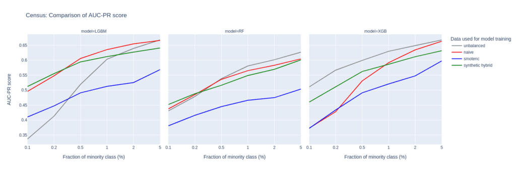
Figure 8: AUC-ROC (top) and AUC-PR (bottom) of classifiers LGBM, RandomForest (RF), and XGB trained on the Census data set to predict the target feature income. The classifiers are trained on unbalanced data sets (grey) and data sets that are upsampled naively (red), with the SMOTE-NC algorithm (blue), and with AI-generated synthetic records (green). AUC values are reported for different fractions of the minority class in the unbalanced training data (x-axis).
Synthetic data for upsampling
AI-based synthetic data generation can provide an effective solution to the problem of highly unbalanced data sets in machine learning. By creating diverse and realistic samples, upsampling with synthetic data generation can improve the performance of predictive models. This is especially true for cases where not only the minority fraction is low but also the absolute number of minority records is at a bare minimum. In such extreme settings, training on data upsampled with AI-generated synthetic records leads to better performance of prediction models than upsampling with SMOTE-NC or naive upsampling. Across all parameter settings explored in this study, synthetic upsampling resulted in predictive models which rank among the top-performing ones.
TABLE OF CONTENT
- Why care about data anonymization tools?
- Data anonymization tools: What are they anyway?
- How do data anonymization tools work?
- Legacy data anonymization approaches
- The next generation of data anonymization tools
- Data anonymization approaches and their use cases
- The best and the worst data anonymization approaches
- Conclusion
Why should you care about data anonymization tools?
Data anonymization tools can be your best friends or your data quality’s worst enemies. Sometimes both. Anonymizing data is never easy, and it gets trickier when:
- You collect more data,
- Your datasets become more complex,
- Your adversaries come up with new types of privacy attacks,
- You remove PII from your data, thinking it will provide privacy protection,
- You add too much noise to the data and destroy the intellingence.
You try to do your best and use data anonymization tools on a daily basis. You have removed all sensitive information, masked the rest, and randomized for good measure. So, your data is safe now. Right?

As the Austrians—Arnold Schwarzenegger included—say: Schmäh! Which roughly translates as bullshit. Why do so many data anonymization efforts end up being Schmäh?
Data anonymization tools: What are they anyway?
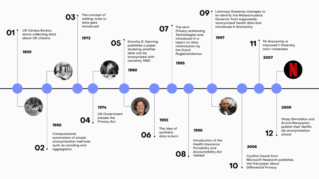
Data anonymization tools conveniently automate the process of data anonymization with the goal of making sure that no individual included in the data can be re-identified. The most ancient of data anonymization tools, namely aggregation and the now obsolete rounding, were born in the 1950s. The concept of adding noise to data as a way to protect anonymity entered the picture in the 1970s. We have come a long way since then. Privacy-enhancing technologies were born in the 90s and have been evolving since, offering better, safer, and more data-friendly data anonymization tools.
Data anonymization tools must constantly evolve since attacks are also getting more and more sophisticated. Today, new types of privacy attacks using the power of AI, can reidentify individuals in datasets that are thought of as anonymous. Data privacy is a constantly shifting field with lots of moving targets and constant pressure to innovate.
Data anonymization tools: How do they work?
Although a myriad of data anonymization tools exist, we can differentiate between two groups of data anonymization tools based on how they approach privacy in principle. Legacy data anonymization tools work by removing or disguising personally identifiable information, or so-called PII. Traditionally, this means unique identifiers, such as social security numbers, credit card numbers, and other kinds of ID numbers.
The trouble with these types of data anonymization tools is that no matter how much of the data is removed or modified, a 1:1 relationship between the data subject and the data points remains. With the advances of AI-based reidentification attacks, it’s getting increasingly easier to find this 1:1 relationship, even in the absence of obvious PII pointers. Our behavior—essentially a series of events—is almost like a fingerprint. An attacker doesn’t need to know my name or social security number if there are other behavior-based identifiers that are unique to me, such as my purchase history or location history. As a result, state of the art data anonymization tools are needed to anonymize behavioral data.
Which data anonymization approaches can be considered legacy?
Legacy data anonymization tools are often associated with manual work, whereas modern data privacy solutions incorporate machine learning and AI to achieve more dynamic and effective results. But let's have a look at the most common forms of traditional anonymization first.
1. What is data masking?
Data masking is one of the most frequently used data anonymization approaches across industries. It works by replacing parts of the original data with asterisks or another placeholder. Data masking can reduce the value or utility of the data, especially if it's too aggressive. The data might not retain the same distribution or characteristics as the original, making it less useful for analysis.
The process of data masking can be complex, especially in environments with large and diverse datasets. The masking should be consistent across all records to ensure that the data remains meaningful. The masked data should adhere to the same validation rules, constraints, and formats as the original dataset. Over time, as systems evolve and new data is added or structures change, ensuring consistent and accurate data masking can become challenging.
The biggest challenge with data masking: to decide what to actually mask. Simply masking PII from data using Python, for example, still has its place, but the resulting data should not be considered anonymized by any stretch of the imagination. The problem are quasi identifiers (= the combination of attributes of data) that if left unprocessed still allow re-identification in a masked dataset quite easily.

2. What is pseudonymization?
Pseudonymization is strictly speaking not an anonymization approach as pseudomized data is not anonymous data. However, it's very common and so we will explain it here. Pseudonymization replaces private identifiers with fake identifiers, or pseudonyms or removes private identifiers alltogether. While the data can still be matched with its source when one has the right key, it can't be matched without it. The 1:1 relationship remains and can be recovered not only by accessing the key but also by linking different datasets. The risk of reversibility is always high, and as a result, pseudonymization should only be used when it’s absolutely necessary to reidentify data subjects at a certain point in time.
The pseudonyms typically need a key for the transformation process. Managing, storing, and protecting this key is critical. If it's compromised, the pseudonymization can be reversed.
What’s more, under GDPR, pseudonymized data is still considered personal data, meaning that data protection obligations continue to apply.
Overall, while pseudonymization might be a common practice today, it should only be used as a stand-alone tool when absolutely necessary. Pseudonymization is not anonymization and pseudonymized data should never be considered anonymized.
3. What is generalization and aggregation?
This method reduces the granularity of the data. For instance, instead of displaying an exact age of 27, the data might be generalized to an age range, like 20-30. Generalization causes a significant loss of data utility by decreasing data granularity. Over-generalizing can render data almost useless, while under-generalizing might not provide sufficient privacy.

You also have to consider the risk of residual disclosure. Generalized data sets might contain enough information to infer about individuals, especially when combined with other data sources.
4. What is data swapping or perturbation?
Data swapping or perturbation describes the approach of replacing original data values with values from other records. The privacy-utility trade-off strikes again: perturbing data leads to a loss of information, which can affect the accuracy and reliability of analyses performed on the perturbed data. However at the same time the achieved privacy protection is not very high. Protecting against re-identification while maintaining data utility is challenging. Finding the appropriate perturbation methods that suit the specific data and use case is not always straightforward.

5. What is randomization?
Randomization is a legacy data anonymization approach that changes the data to make it less connected to a person. This is done through adding random noise to the data.
Some data types, such as geospatial or temporal data, can be challenging to randomize effectively while maintaining data utility. Preserving spatial or temporal relationships in the data can be complex.
Selecting the right approach (i.e. what variables to add noise to and how much) to do the job is also challenging since each data type and use case could call for a different approach. Choosing the wrong approach can have serious consequences downstream, resulting in inadequate privacy protection or excessive data distortion.
Data consumers could be unaware of the effect randomization had on the data and might end up with false conclusions. On the bright side, randomization techniques are relatively straightforward to implement, making them accessible to a wide range of organizations and data professionals.
6. What is data redaction?
Data redaction is similar to data masking, but in the case of this data anonymization approach, entire data values or sections are removed or obscured. Deleting PII is easy to do. However, it’s a sure-fire way to encounter a privacy disaster down the line. It’s also devastating for data utility since critical elements or crucial contextual information could be removed from the data.

Redacted data may introduce inconsistencies or gaps in the dataset, potentially affecting data integrity. Redacting sensitive information can result in a smaller dataset. This could impact statistical analyses and models that rely on a certain volume of data for accuracy.
Next-generation data anonymization tools
The next-generation data anonymization tools, or so-called privacy-enhancing technologies take an entirely different, more use-case-centered approach to data anonymization and privacy protection.
1. Homomorphic encryption
The first group of modern data anonymization tools works by encrypting data in a way that allows for computational operations on encrypted data. The downside of this approach is that the data, well, stays encrypted which makes it very hard to work with such data if it was previously unknown the user. You can't perform e.g. exploratory analyses on encrypted data. In addition it is computationally very intensive and, as such, not widely available and cumbersome to use. As the price of computing power decreases and capacity increases, this technology is set to become more popular and easier to access.
2. Federated learning
Federated learning is a fairly complicated approach, enabling machine learning models to be trained on distributed datasets. Federated learning is commonly used in applications that involve mobile devices, such as smartphones and IoT devices.
For example, predictive text suggestions on smartphones can be improved without sending individual typing data to a central server. In the energy sector, federated learning helps optimize energy consumption and distribution without revealing specific consumption patterns of individual users or entities. However, these federated systems require the participation of all players, which is near-impossible to achieve if the different parts of the system belong to different operators. Simply put, Google can pull it off, while your average corporation would find it difficult.
3. Synthetic data generation
A more readily available approach is an AI-powered data anonymization tool: synthetic data generation. Synthetic data generation extracts the distributions, statistical properties, and correlations of datasets and generates entirely new, synthetic versions of said datasets, where all individual data points are synthetic. The synthetic data points look realistic and, on a group level, behave like the original. As a data anonymization tool, reliable synthetic data generators produce synthetic data that is representative, scalable, and suitable for advanced use cases, such as AI and machine learning development, analytics, and research collaborations.
4. Secure multiparty computation (SMPC)
Secure Multiparty Computation (SMPC), in simple terms, is a cryptographic technique that allows multiple parties to jointly compute a function over their private inputs while keeping those inputs confidential. It enables these parties to collaborate and obtain results without revealing sensitive information to each other.
While it's a powerful tool for privacy-preserving computations, it comes with its set of implementation challenges, particularly in terms of complexity, efficiency, and security considerations. It requires expertise and careful planning to ensure that it is applied effectively and securely in practical applications.

Data anonymization approaches and their use cases
Data anonymization encompass a diverse set of approaches, each with its own strengths and limitations. In this comprehensive guide, we explore ten key data anonymization strategies, ranging from legacy methods like data masking and pseudonymization to cutting-edge approaches such as federated learning and synthetic data generation. Whether you're a data scientist or privacy officer, you will find this bullshit-free table listing their advantages, disadvantages, and common use cases very helpful.
| # | Data Anonymization Approach | Description | Advantages | Disadvantages | Use Cases |
|---|---|---|---|---|---|
| 1 | Data Masking | Masks or disguises sensitive data by replacing characters with symbols or placeholders. | - Simplicity of implementation. - Preservation of data structure. | - Limited protection against inference attacks. - Potential negative impact on data analysis. | - Anonymizing email addresses in communication logs. - Concealing rare names in datasets. - Masking sensitive words in text documents. |
| 2 | Pseudonymization | Replaces sensitive data with pseudonyms or aliases or removes it alltogether. | - Preservation of data structure. - Data utility is generally preserved. - Fine-grained control over pseudonymization rules. | - Pseudomized data is not anonymous data. - Risk of re-identification is very high. - Requires secure management of pseudonym mappings. | - Protecting patient identities in medical research. - Securing employee IDs in HR records. |
| 3 | Generalization/Aggregation | Aggregates or generalizes data to reduce granularity. | - Simple implementation. | - Loss of fine-grained detail in the data. - Risk of data distortion that affects analysis outcomes. - Challenging to determine appropriate levels of generalization. | - Anonymizing age groups in demographic data. - Concealing income brackets in economic research. |
| 4 | Data Swapping/Perturbation | Swaps or perturbs data values between records to break the link between individuals and their data. | - Flexibility in choosing perturbation methods. - Potential for fine-grained control. | - Privacy-utility trade-off is challenging to balance. - Risk of introducing bias in analyses. - Selection of appropriate perturbation methods is crucial. | - E-commerce. - Online user behavior analysis. |
| 5 | Randomization | Introduces randomness (noise) into the data to protect data subjects. | - Flexibility in applying to various data types. - Reproducibility of results when using defined algorithms and seeds. | - Privacy-utility trade-off is challenging to balance. - Risk of introducing bias in analyses. - Selection of appropriate randomization methods is hard. | - Anonymizing survey responses in social science research. - Online user behavior analysis. |
| 6 | Data Redaction | Removes or obscures specific parts of the dataset containing sensitive information. | - Simplicity of implementation. | - Loss of data utility, potentially significant. - Risk of removing contextual information. - Data integrity challenges. | - Concealing personal information in legal documents. - Removing private data in text documents. |
| 7 | Homomorphic Encryption | Encrypts data in such a way that computations can be performed on the encrypted data without decrypting it, preserving privacy. | - Strong privacy protection for computations on encrypted data. - Supports secure data processing in untrusted environments. - Cryptographically provable privacy guarantees. | - Encrypted data cannot be easily worked with if previously unknown to the user. - Complexity of encryption and decryption operations. - Performance overhead for cryptographic operations. - May require specialized libraries and expertise. | - Basic data analytics in cloud computing environments. - Privacy-preserving machine learning on sensitive data. |
| 8 | Federated Learning | Trains machine learning models across decentralized edge devices or servers holding local data samples, avoiding centralized data sharing. | - Preserves data locality and privacy, reducing data transfer. - Supports collaborative model training on distributed data. - Suitable for privacy-sensitive applications. | - Complexity of coordination among edge devices or servers. - Potential communication overhead. - Ensuring model convergence can be challenging. - Shared models can still leak privacy. | - Healthcare institutions collaboratively training disease prediction models. - Federated learning for mobile applications preserving user data privacy. - Privacy-preserving AI in smart cities. |
| 9 | Synthetic Data Generation | Creates artificial data that mimics the statistical properties of the original data while protecting privacy. | - Strong privacy protection with high data utility. - Preserves data structure and relationships. - Scalable for generating large datasets. | - Accuracy and representativeness of synthetic data may vary depending on the generator. - May require specialized algorithms and expertise. | - Sharing synthetic healthcare data for research purposes. - Synthetic data for machine learning model training. - Privacy-preserving data sharing in financial analysis. |
| 10 | Secure Multiparty Computation (SMPC) | Enables multiple parties to jointly compute functions on their private inputs without revealing those inputs to each other, preserving privacy. | - Strong privacy protection for collaborative computations. - Suitable for multi-party data analysis while maintaining privacy. - Offers security against collusion. | - Complexity of protocol design and setup. - Performance overhead, especially for large-scale computations. - Requires trust in the security of the computation protocol. | - Privacy-preserving data aggregation across organizations. - Collaborative analytics involving sensitive data from multiple sources. - Secure voting systems. |
The best and the worst data anonymization approaches
When it comes to choosing the right data anonymization approach, we are faced with a complex problem requiring a nuanced view and careful consideration. When we put all the Schmäh aside, choosing the right data anonymization strategy comes down to balancing the so-called privacy-utility trade-off.

The privacy-utility trade-off refers to the balancing act of data anonymization’ two key objectives: providing privacy to data subjects and utility to data consumers. Depending on the specific use case, the quality of implementation, and the level of privacy required, different data anonymization approaches are more or less suitable to achieve the ideal balance of privacy and utility. However, some data anonymization approaches are inherently better than others when it comes to the privacy-utility trade-off. High utility with robust, unbreakable privacy is the unicorn all privacy officers are hunting for, and since the field is constantly evolving with new types of privacy attacks, data anonymization must evolve too.
As it stands today, the best data anonymization approaches for preserving a high level of utility while effectively protecting privacy are the following:
Synthetic Data Generation
Synthetic data generation techniques create artificial datasets that mimic the statistical properties of the original data. These datasets can be shared without privacy concerns. When properly designed, synthetic data can preserve data utility for a wide range of statistical analyses while providing strong privacy protection. It is particularly useful for sharing data for research and analysis without exposing sensitive information.
Privacy: high
Utility: high for analytical, data sharing, and ML/AI training use cases
Homomorphic Encryption
Homomorphic encryption allows computations to be performed on encrypted data without the need to decrypt it. This technology is valuable for secure data processing in untrusted environments, such as cloud computing. While it can be computationally intensive, it offers a high level of privacy and maintains data utility for specific tasks, particularly when privacy-preserving machine learning or data analytics is involved. Depending on the specific encryption scheme and parameters chosen, there may be a trade-off between the level of security and the efficiency of computations. Also, increasing security often leads to slower performance.
Privacy: high
Utility: can be high, depending on the use case
Secure Multiparty Computation (SMPC)
SMPC allows multiple parties to jointly compute a function over their private inputs without revealing those inputs to each other. It offers strong privacy guarantees and can be used for various collaborative data analysis tasks while preserving data utility. SMPC has applications in areas like secure data aggregation and privacy-preserving collaborative analytics.
Privacy: High
Utility: can be high, depending on the use case
Data anonymization tools: the saga continues
In the ever-evolving landscape of data anonymization strategies, the journey to strike a balance between preserving privacy and maintaining data utility is an ongoing challenge. As data grows more extensive and complex and adversaries devise new tactics, the stakes of protecting sensitive information have never been higher.
Legacy data anonymization approaches have their limitations and are increasingly likely to fail in protecting privacy. While they may offer simplicity in implementation, they often fall short in preserving the intricate relationships and structures within data.
Modern data anonymization tools, however, present a promising shift towards more robust privacy protection. Privacy-enhancing technologies have emerged as powerful solutions. These tools harness encryption, machine learning, and advanced statistical techniques to safeguard data while enabling meaningful analysis.
Furthermore, the rise of synthetic data generation signifies a transformative approach to data anonymization. By creating artificial data that mirrors the statistical properties of the original while safeguarding privacy, synthetic data generation provides an innovative solution for diverse use cases, from healthcare research to machine learning model training.
As the data privacy landscape continues to evolve, organizations must stay ahead of the curve. What is clear is that the pursuit of privacy-preserving data practices is not only a necessity but also a vital component of responsible data management in our increasingly vulnerable world.
In this tutorial, you will learn how to use synthetic rebalancing to improve the performance of machine-learning (ML) models on imbalanced classification problems. Rebalancing can be useful when you want to learn more of an otherwise small or underrepresented population segment by generating more examples of it. Specifically, we will look at classification ML applications in which the minority class accounts for less than 0.1% of the data.
We will start with a heavily imbalanced dataset. We will use synthetic rebalancing to create more high-quality, statistically representative instances of the minority class. We will compare this method against 2 other types of rebalancing to explore their advantages and pitfalls. We will then train a downstream machine learning model on each of the rebalanced datasets and evaluate their relative predictive performance. The Python code for this tutorial is publicly available and runnable in this Google Colab notebook.
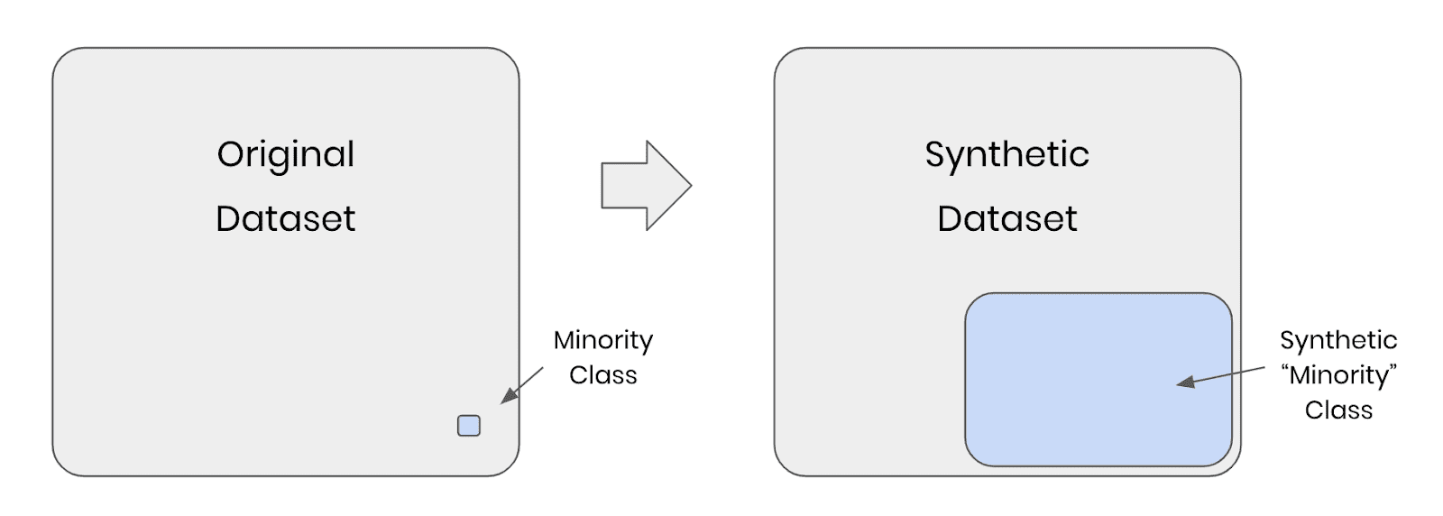
Fig 1 - Synthetic rebalancing creates more statistically representative instances of the minority class
Why should I rebalance my dataset?
In heavily imbalanced classification projects, a machine learning model has very little data to effectively learn patterns about the minority class. This will affect its ability to correctly class instances of this minority class in the real (non-training) data when the model is put into production. A common real-world example is credit card fraud detection: the overwhelming majority of credit card transactions are perfectly legitimate, but it is precisely the rare occurrences of illegitimate use that we would be interested in capturing.
Let’s say we have a training dataset with 100,000 credit card transactions which contains 999,900 legitimate transactions and 100 fraudulent ones. A machine-learning model trained on this dataset would have ample opportunity to learn about all the different kinds of legitimate transactions, but only a small sample of 100 records in which to learn everything it can about fraudulent behavior. Once this model is put into production, the probability is high that fraudulent transactions will occur that do not follow any of the patterns seen in the small training sample of 100 fraudulent records. The machine learning model is unlikely to classify these fraudulent transactions.
So how can we address this problem? We need to give our machine learning model more examples of fraudulent transactions in order to ensure optimal predictive performance in production. This can be achieved through rebalancing.
Rebalancing Methods
We will explore three types of rebalancing:
- Random (or “naive”) oversampling
- SMOTE upsampling
- Synthetic rebalancing
The tutorial will give you hands-on experience with each type of rebalancing and provide you with in-depth understanding of the differences between them so you can choose the right method for your use case. We’ll start by generating an imbalanced dataset and showing you how to perform synthetic rebalancing using MOSTLY AI's synthetic data generator. We will then compare performance metrics of each rebalancing method on a downstream ML task.
But first things first: we need some data.
Generate an Imbalanced Dataset
For this tutorial, we will be using the UCI Adult Income dataset, as well as the same training and validation split, that was used in the Train-Synthetic-Test-Real tutorial. However, for this tutorial we will work with an artificially imbalanced version of the dataset containing only 0.1% of high-income (>50K) records in the training data, by downsampling the minority class. The downsampling has already been done for you, but if you want to reproduce it yourself you can use the code block below:
def create_imbalance(df, target, ratio):
    val_min, val_maj = df[target].value_counts().sort_values().index
    df_maj = df.loc[df[target]==val_maj]
    n_min = int(df_maj.shape[0]/(1-ratio)*ratio)
    df_min = df.loc[df[target]==val_min].sample(n=n_min, random_state=1)
    df_maj = df.loc[df[target]==val_maj]
    df_imb = pd.concat([df_min, df_maj]).sample(frac=1, random_state=1)
    return df_imb

df_trn = pd.read_csv(f'{repo}/census-training.csv')
df_trn_imb = create_imbalance(df_trn, 'income', 1/1000)
df_trn_imb.to_csv('census-training-imbalanced.csv', index=False)
Let’s take a quick look at this imbalanced dataset by randomly sampling 10 rows. For legibility let’s select only a few columns, including the income column as our imbalanced feature of interest:
trn = pd.read_csv(f'{repo}/census-training-imbalanced.csv')
trn.sample(n=10)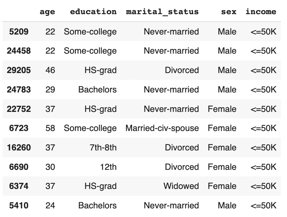
You can try executing the line above multiple times to see different samples. Still, due to the strong class imbalance, the chance of finding a record with high income in a random sample of 10 is minimal. This would be problematic if you were interested in creating a machine learning model that could accurately classify high-income records (which is precisely what we’ll be doing in just a few minutes).
The problem becomes even more clear when we try to sample a specific sub-group in the population. Let’s sample all the female doctorates with a high income in the dataset. Remember, the dataset contains almost 30 thousand records.
trn[
    (trn['income']=='>50K')
    & (trn.sex=='Female')
    & (trn.education=='Doctorate')
]
It turns out there are actually no records of this type in the training data. Of course, we know that these kinds of individuals exist in the real world and so our machine learning model is likely to encounter them when put in production. But having had no instances of this record type in the training data, it is likely that the ML model will fail to classify this kind of record correctly. We need to provide the ML model with a higher quantity and more varied range of training samples of the minority class to remedy this problem.
Synthetic rebalancing with MOSTLY AI
MOSTLY AI offers a synthetic rebalancing feature that can be used with any categorical column. Let’s walk through how this works:
- Download the imbalanced dataset here if you haven’t generated it yourself already. Use Ctrl+S or Cmd+S to save the file locally.
- Go to your MOSTLY AI account and navigate to “Synthetic Datasets”. Upload
census-training-imbalanced.csvand click “Proceed”.
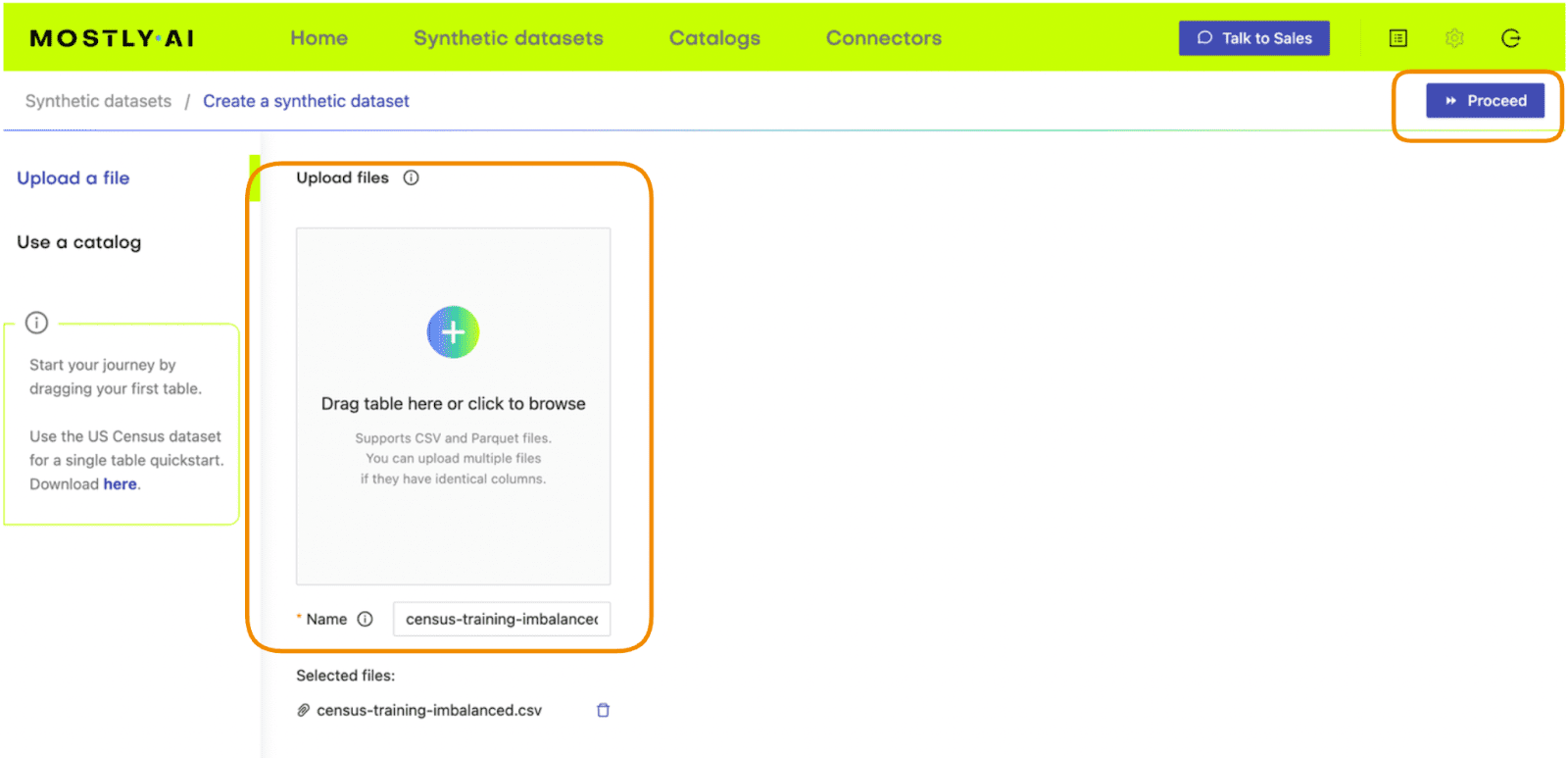
Fig 2 - Upload the original dataset to MOSTLY AI’s synthetic data generator.
- On the next page, click “Data Settings” and then click on the “Income” column
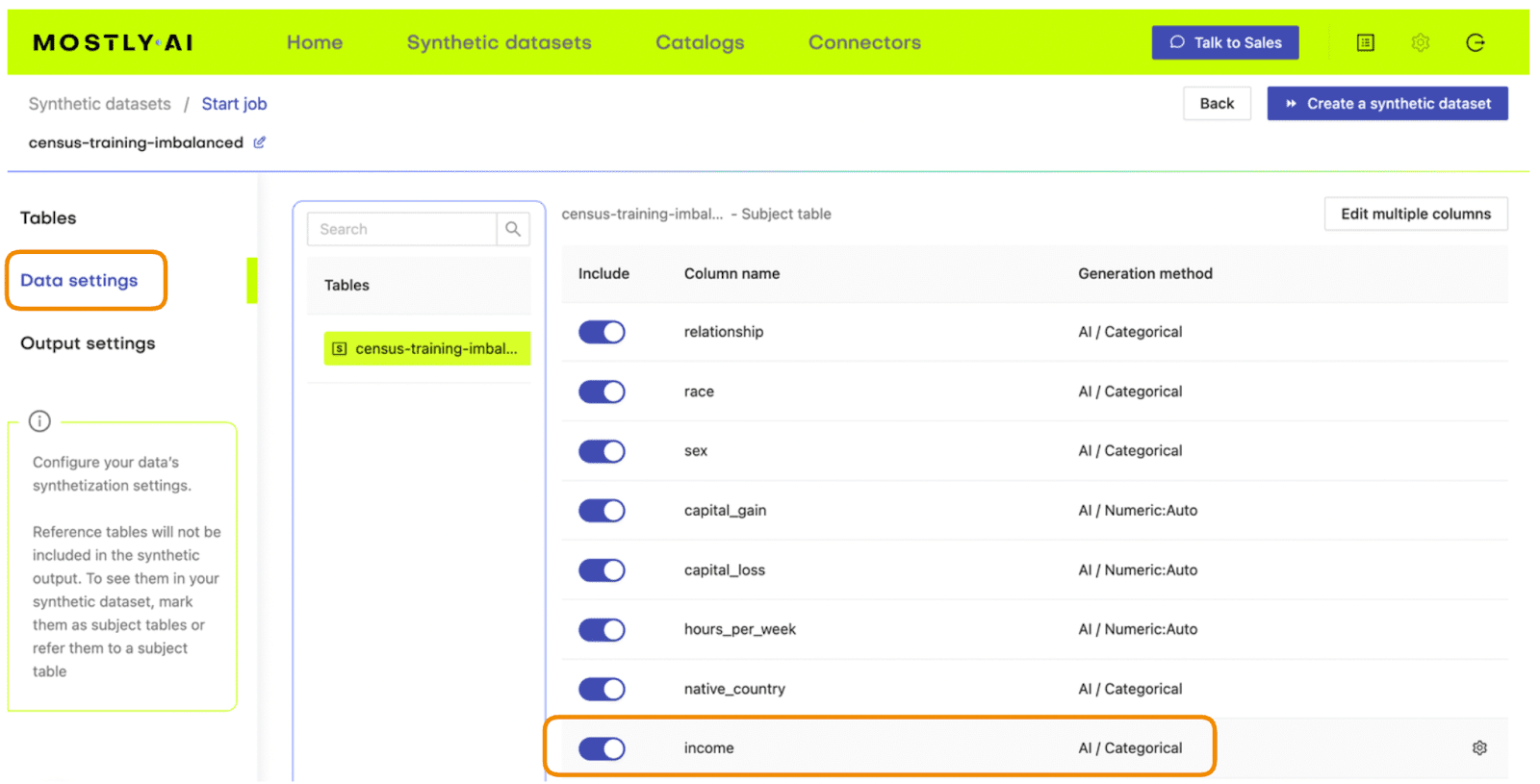
Fig 3 - Navigate to the Data Settings of the Income column.
- Set the Encoding Type to “Categorical” and select the option to “Use this column to rebalance the table”. Then add a new row and rebalance the “>50K” column to be “50%” of the dataset. This will synthetically upsample the minority class to create an even split between high-income and low-income records.
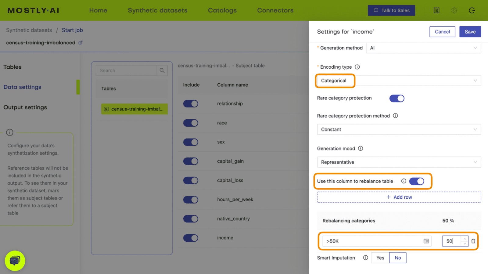
Fig 4 - Set the relevant settings to rebalance the income column.
- Click “Save” and on the next page click “Create a synthetic dataset” to launch the job.

Fig 5 - Launch the synthetic data generation
Once the synthesization is complete, you can download the synthetic dataset to disk. Then return to wherever you are running your code and use the following code block to create a DataFrame containing the synthetic data.
# upload synthetic dataset
import pandas as pd

try:
    # check whether we are in Google colab
    from google.colab import files
    print("running in COLAB mode")
    repo = 'https://github.com/mostly-ai/mostly-tutorials/raw/dev/rebalancing'
    import io
    uploaded = files.upload()
    syn = pd.read_csv(io.BytesIO(list(uploaded.values())[0]))
    print(f"uploaded synthetic data with {syn.shape[0]:,} records and {syn.shape[1]:,} attributes")
except:
    print("running in LOCAL mode")
    repo = '.'
    print("adapt `syn_file_path` to point to your generated synthetic data file")
    syn_file_path = './census-synthetic-balanced.csv'
    syn = pd.read_csv(syn_file_path)
    print(f"read synthetic data with {syn.shape[0]:,} records and {syn.shape[1]:,} attributes")
Let's now repeat the data exploration steps we performed above with the original, imbalanced dataset. First, let’s display 10 randomly sampled synthetic records. We'll subset again for legibility. You can run this line multiple times to get different samples.
# sample 10 random records
syn_sub = syn[['age','education','marital_status','sex','income']]
syn_sub.sample(n=10)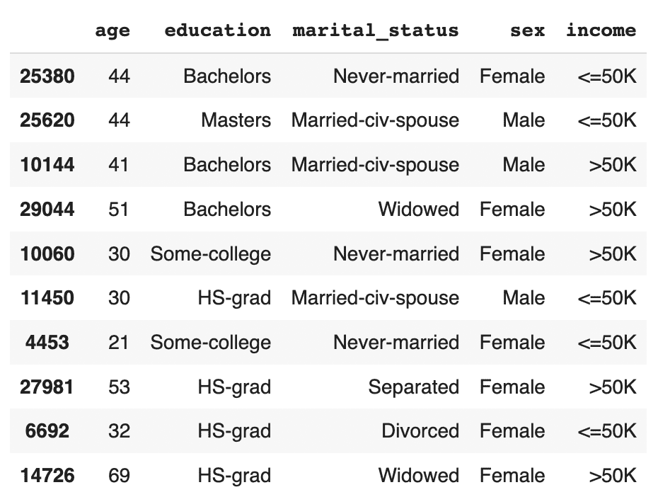
This time, you should see that the records are evenly distributed across the two income classes.
Let's now investigate all female doctorates with a high income in the synthetic, rebalanced dataset:
syn_sub[
    (syn_sub['income']=='>50K')
    & (syn_sub.sex=='Female')
    & (syn_sub.education=='Doctorate')
].sample(n=10)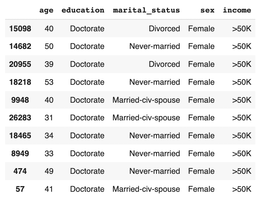
The synthetic data contains a list of realistic, statistically sound female doctorates with a high income. This is great news for our machine learning use case because it means that our ML model will have plenty of data to learn about this particular important subsegment.
Evaluate ML performance using TSTR
Let’s now compare the quality of different rebalancing methods by training a machine learning model on the rebalanced data and evaluating the predictive performance of the resulting models.
We will investigate and compare 3 types of rebalancing:
- Random (or “naive”) oversampling
- SMOTE upsampling
- Synthetic rebalancing
The code block below defines the functions that will preprocess your data, train a LightGBM model and evaluate its performance using a holdout dataset. For more detailed descriptions of this code, take a look at the Train-Synthetic-Test-Real tutorial.
# import necessary libraries
import lightgbm as lgb
from lightgbm import early_stopping
from sklearn.model_selection import train_test_split
from sklearn.metrics import roc_auc_score, f1_score
import seaborn as sns
import matplotlib.pyplot as plt

# define target column and value
target_col = 'income'
target_val = '>50K'

# define preprocessing function
def prepare_xy(df: pd.DataFrame):
    y = (df[target_col]==target_val).astype(int)
    str_cols = [
        col for col in df.select_dtypes(['object', 'string']).columns if col != target_col
    ]
    for col in str_cols:
        df[col] = pd.Categorical(df[col])
    cat_cols = [
        col for col in df.select_dtypes('category').columns if col != target_col
    ]
    num_cols = [
        col for col in df.select_dtypes('number').columns if col != target_col
    ]
    for col in num_cols:
        df[col] = df[col].astype('float')
    X = df[cat_cols + num_cols]
    return X, y

# define training function
def train_model(X, y):
    cat_cols = list(X.select_dtypes('category').columns)
    X_trn, X_val, y_trn, y_val = train_test_split(X, y, test_size=0.2, random_state=1)
    ds_trn = lgb.Dataset(
        X_trn,
        label=y_trn,
        categorical_feature=cat_cols,
        free_raw_data=False
    )
    ds_val = lgb.Dataset(
        X_val,
        label=y_val,
        categorical_feature=cat_cols,
        free_raw_data=False
    )
    model = lgb.train(
        params={
            'verbose': -1,
            'metric': 'auc',
            'objective': 'binary'
         },
         train_set=ds_trn,
         valid_sets=[ds_val],
         callbacks=[early_stopping(5)],
    )
    return model

# define evaluation function
def evaluate_model(model, hol):
    X_hol, y_hol = prepare_xy(hol)
    probs = model.predict(X_hol)
    preds = (probs >= 0.5).astype(int)
    auc = roc_auc_score(y_hol, probs)
    f1 = f1_score(y_hol, probs>0.5, average='macro')
    probs_df = pd.concat([
        pd.Series(probs, name='probability').reset_index(drop=True),
        pd.Series(y_hol, name=target_col).reset_index(drop=True)
    ], axis=1)
    sns.displot(
        data=probs_df,
        x='probability',
        hue=target_col,
        bins=20,
        multiple="stack"
     )
    plt.title(f"AUC: {auc:.1%}, F1 Score: {f1:.2f}", fontsize = 20)
    plt.show()
    return auc

# create holdout dataset
df_hol = pd.read_csv(f'{repo}/census-holdout.csv')
df_hol_min = df_hol.loc[df_hol['income']=='>50K']
print(f"Holdout data consists of {df_hol.shape[0]:,} records",
f"with {df_hol_min.shape[0]:,} samples from the minority class")
ML performance of imbalanced dataset
Let’s now train a LightGBM model on the original, heavily imbalanced dataset and evaluate its predictive performance. This will give us a baseline against which we can compare the performance of the different rebalanced datasets.
X_trn, y_trn = prepare_xy(trn)
model_trn = train_model(X_trn, y_trn)
auc_trn = evaluate_model(model_trn, df_hol)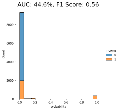
With an AUC of about 50%, the model trained on the imbalanced dataset is just as good as a flip of a coin, or, in other words, not worth very much at all. The downstream LightGBM model is not able to learn any signal due to the low number of minority-class samples.
Let’s see if we can improve this using rebalancing.
Naive rebalancing
First, let’s rebalance the dataset using the random oversampling method, also known as “naive rebalancing”. This method simply takes the minority class records and copies them to increase their quantity. This increases the number of records of the minority class but does not increase the statistical diversity. We will use the imblearn library to perform this step, feel free to check out their documentation for more context.
The code block performs the naive rebalancing, trains a LightGBM model using the rebalanced dataset and evaluates its predictive performance:
from imblearn.over_sampling import RandomOverSampler

X_trn, y_trn = prepare_xy(trn)
sm = RandomOverSampler(random_state=1)
X_trn_up, y_trn_up = sm.fit_resample(X_trn, y_trn)
model_trn_up = train_model(X_trn_up, y_trn_up)
auc_trn_up = evaluate_model(model_trn_up, df_hol)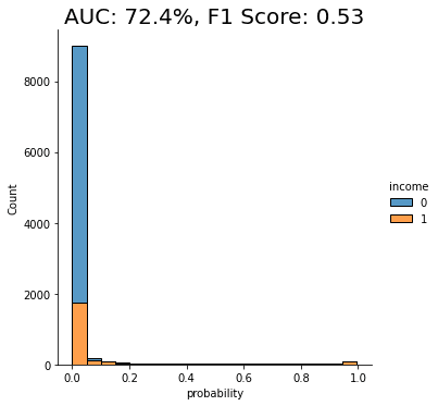
We see a clear improvement in predictive performance, with an AUC score of around 70%. This is better than the baseline model trained on the imbalanced dataset, but still not great. We see that a significant portion of the “0” class (low-income) is being incorrectly classified as “1” (high-income).
This is not surprising because, as stated above, this rebalancing method just copies the existing minority class records. This increases their quantity but does not add any new statistical information into the model and therefore does not offer the model much data that it can use to learn about minority-class instances that are not present in the training data.
Let’s see if we can improve on this using another rebalancing method.
SMOTE rebalancing
SMOTE upsampling is a state-of-the art upsampling method which, unlike the random oversampling seen above, does create novel, statistically representative samples. It does so by interpolating between neighboring samples. It’s important to note, however, that SMOTE upsampling is non-privacy-preserving.
The following code block performs the rebalancing using SMOTE upsampling, trains a LightGBM model on the rebalanced dataset, and evaluates its performance:
from imblearn.over_sampling import SMOTENC

X_trn, y_trn = prepare_xy(trn)
sm = SMOTENC(
    categorical_features=X_trn.dtypes=='category',
    random_state=1
)
X_trn_smote, y_trn_smote = sm.fit_resample(X_trn, y_trn)
model_trn_smote = train_model(X_trn_smote, y_trn_smote)
auc_trn_smote = evaluate_model(model_trn_smote, df_hol)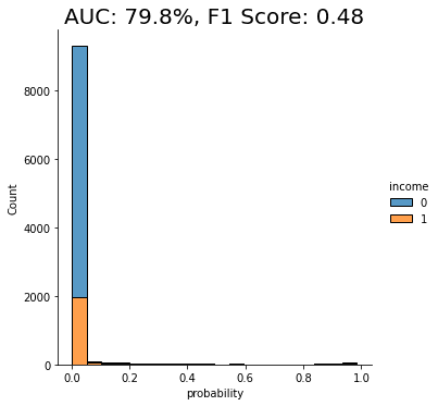
We see another clear jump in performance: the SMOTE upsampling boosts the performance of the downstream model to close to 80%. This is clearly an improvement from the random oversampling we saw above, and for this reason, SMOTE is quite commonly used.
Let’s see if we can do even better.
Synthetic rebalancing with MOSTLY AI
In this final step, let’s take the synthetically rebalanced dataset that we generated earlier using MOSTLY AI to train a LightGBM model. We’ll then evaluate the performance of this downstream ML model and compare it against those we saw above.
The code block below prepares the synthetically rebalanced data, trains the LightGBM model, and evaluates it:
X_syn, y_syn = prepare_xy(syn)
model_syn = train_model(X_syn, y_syn)
auc_syn = evaluate_model(model_syn, df_hol)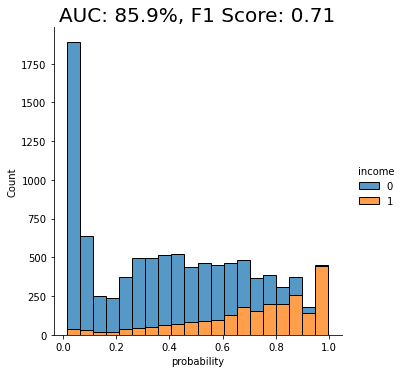
Both performance measures, the AUC as well as the macro-averaged F1 score, are significantly better for the model that was trained on synthetic data than if it were trained on any of the other methods. We can also see that the portion of “0”s incorrectly classified as “1”s has dropped significantly.
The synthetically rebalanced dataset has enabled the model to make fine-grained distinctions between the high-income and low-income records. This is strong proof of the value of synthetic rebalancing for learning more about a small sub-group within the population.
The value of synthetic rebalancing
In this tutorial, you have seen firsthand the value of synthetic rebalancing for downstream ML classification problems. You have gained an understanding of the necessity of rebalancing when working with imbalanced datasets in order to provide the machine learning model with more samples of the minority class. You have learned how to perform synthetic rebalancing with MOSTLY AI and observed the superior performance of this rebalancing method when compared against other methods on the same dataset. Of course, the actual lift in performance may vary depending on the dataset, the predictive task, and the chosen ML model.
What’s next?
In addition to walking through the above instructions, we suggest experimenting with the following in order to get an even better grasp of synthetic rebalancing:
- repeat the experiments for different class imbalances,
- repeat the experiments for different datasets, ML models, and predictive tasks.
In this tutorial, you will explore the relationship between the size of your training sample and synthetic data accuracy. This is an important concept to master because it can help you significantly reduce the runtime and computational cost of your training runs while maintaining the optimal accuracy you require.
We will start with a single real dataset, which we will use to create 5 different synthetic datasets, each with a different training sample size. We will then evaluate the accuracy of the 5 resulting synthetic datasets by looking at individual variable distributions, by verifying rule-adherence and by evaluating their performance on a downstream machine-learning (ML) task. The Python code for this tutorial is runnable and publicly available in this Google Colab notebook.
Size vs synthetic data accuracy tradeoff
Our working hypothesis is that synthetic data accuracy will increase as the number of training samples increases: the more data the generative AI model has to learn from, the better it will perform.
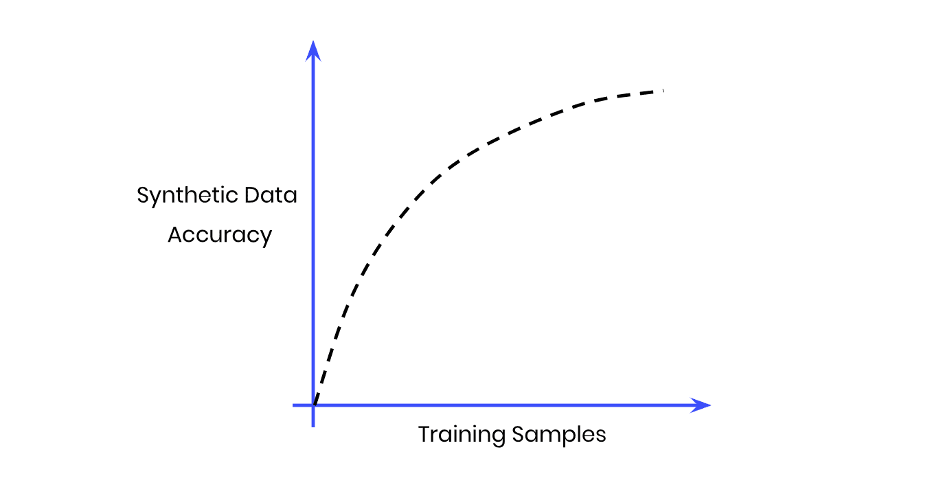
Fig 1 - The Size vs Accuracy Tradeoff
But more training samples also means more data to crunch; i.e. more computational cost and a longer runtime. Our goal, then, will be to find the sweet spot at which we achieve optimal accuracy with the lowest number of training samples possible.
Note that we do not expect synthetic data to ever perfectly match the original data. This would only be satisfied by a copy of the data, which obviously would neither satisfy any privacy requirements nor would provide any novel samples. That being said, we shall expect that due to sampling variance the synthetic data can deviate. Ideally this deviation will be just as much, and not more, than the deviation that we would observe by analyzing an actual holdout dataset.
Synthesize your data
For this tutorial, we will be using the same UCI Adult Income dataset, as well as the same training and validation split, that was used in the Train-Synthetic-Test-Real tutorial. This means we have a total of 48,842 records across 15 attributes, and will be using up to 39,074 (=80%) of those records for the synthesis.
- Download the training data
census-training.csvby clicking here and pressing Ctrl+S or Cmd+S to save the file locally. This is an 80% sample of the full dataset. The remaining 20% sample (which we’ll use for evaluation later) can be fetched from here.
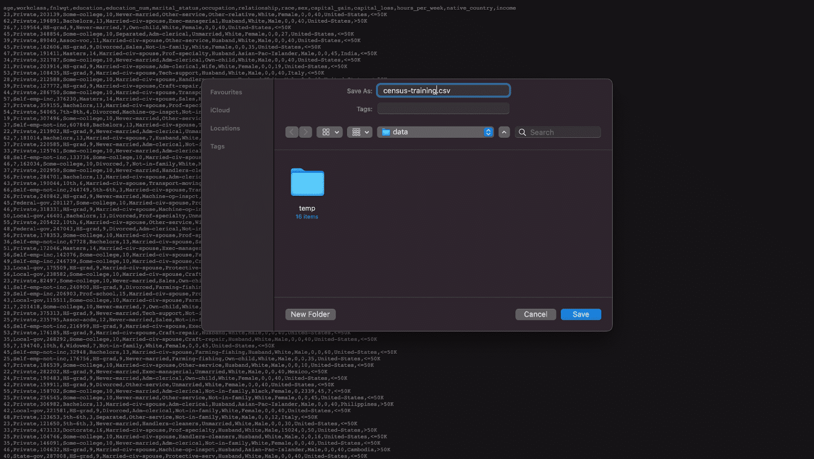
Fig 2 - Download the original training data and save it to disk.
- Synthesize census-training.csv via MOSTLY AI's synthetic data generator multiple times, each time with a different number of maximum training samples. We will use the following training sample sizes in this tutorial: 100, 400, 1600, 6400, 25600. Always generate a consistent number of subjects, e.g. 10,000. You can leave all other settings at their default.
- Download the generated datasets from MOSTLY AI as CSV files, and rename each CSV file with an appropriate name (eg. syn_00100.csv, syn_00400.csv, etc.)
- Now ensure you can access the synthetic datasets from wherever you are running the code for this tutorial. If you are working from the Colab notebook, you can upload the synthetic datasets by executing the code block below:
# upload synthetic dataset
import pandas as pd
try:
    # check whether we are in Google colab
    from google.colab import files
    print("running in COLAB mode")
    repo = 'https://github.com/mostly-ai/mostly-tutorials/raw/dev/size-vs-accuracy'
    import io
    uploaded = files.upload()
    synthetic_datasets = {
        file_name: pd.read_csv(io.BytesIO(uploaded[file_name]), skipinitialspace=True)
        for file_name in uploaded
    }
except:
    print("running in LOCAL mode")
    repo = '.'
    print("upload your synthetic data files to this directory via Jupyter")
    from pathlib import Path
    syn_files = sorted(list(Path('.').glob('syn*csv')))
    synthetic_datasets = {
        file_name.name: pd.read_csv(file_name)
        for file_name in syn_files
    }


for k, df in synthetic_datasets.items():
    print(f"Loaded Dataset `{k}` with {df.shape[0]:,} records and {df.shape[1]:,} attributes")
Evaluate synthetic data accuracy
Now that you have your 5 synthetic datasets (each trained on a different training sample size) let’s take a look at the high-level accuracy scores of these synthetic datasets.
- Navigate to your MOSTLY AI account and note the reported overall synthetic data accuracy as well as the runtime of each job:
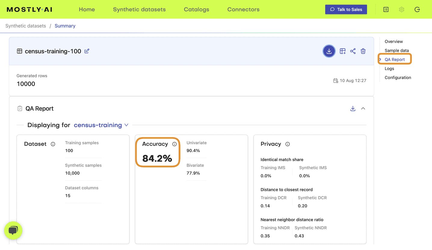
Fig 3 - Note the accuracy score in the QA Report tab of your completed synthetic dataset job.
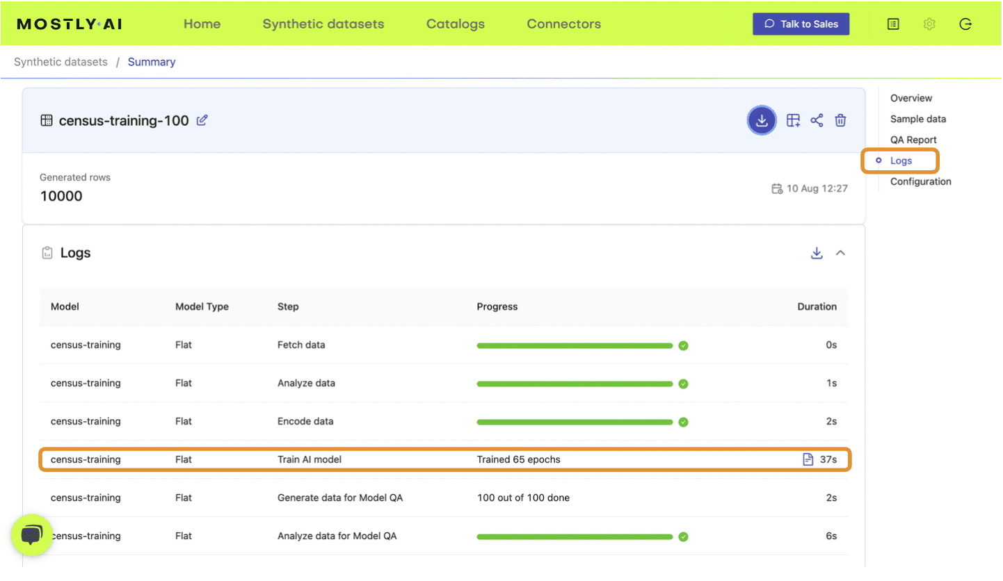
Fig 4 - Note the training time from the Logs tab.
- Update the following DataFrame accordingly:
results = pd.DataFrame([
{'file': 'syn_00100.csv', 'samples': 100, 'accuracy': 0.830, 'runtime': 37},
{'file': 'syn_00400.csv', 'samples': 400, 'accuracy': 0.914, 'runtime': 45},
{'file': 'syn_01600.csv', 'samples': 1600, 'accuracy': 0.956, 'runtime': 48},
{'file': 'syn_06400.csv', 'samples': 6400, 'accuracy': 0.972, 'runtime': 54},
{'file': 'syn_25600.csv', 'samples': 25600, 'accuracy': 0.980, 'runtime': 75},
])
results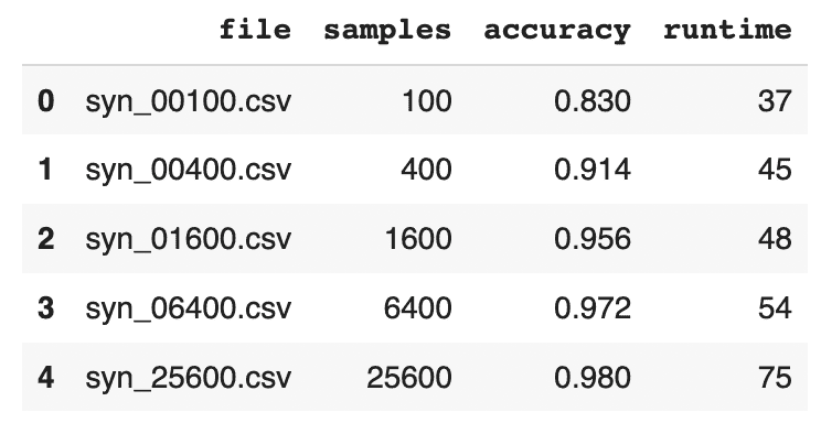
- Visualize the results using the code block below:
import seaborn as sns
import matplotlib.pyplot as plt

sns.catplot(data=results, y='accuracy', x='file', kind='point', color='black')
plt.xticks(rotation=45)
plt.xlabel('')
plt.title('QA Report - Overall Accuracy')
plt.show()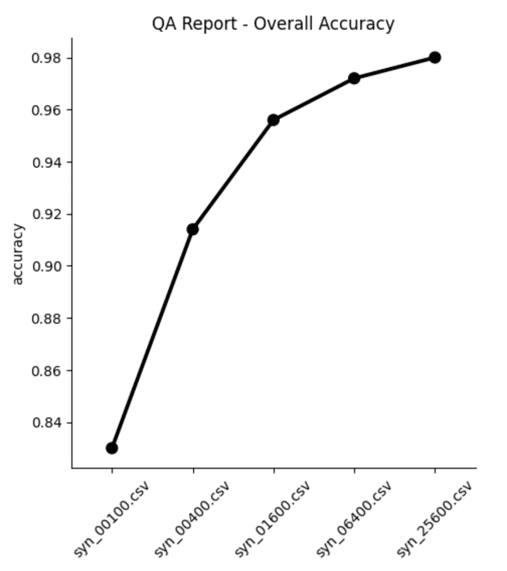
From both the table and the plot we can see that, as expected, the overall accuracy of the synthetic data improves as we increase the number of training samples. But notice that the increase is not strictly linear: while we see big jumps in accuracy performance between the first three datasets (100, 400 and 1,600 samples, respectively), the jumps get smaller as the training samples increase in size. Between the last two datasets (trained on 6,400 and 25,600 samples, respectively) the increase in accuracy is less than 0.1%, while the runtime increases by more than 35%.
Synthetic data quality deep-dive
The overall accuracy score is a great place to start when assessing the quality of your synthetic data, but let’s now dig a little deeper to see how the synthetic dataset compares to the original data from a few different angles. We’ll take a look at:
- Distributions of individual variables
- Rule adherence
- Performance on a downstream ML task
Before you jump into the next sections, run the code block below to concatenate all the 5 synthetic datasets together in order to facilitate comparison:
# combine synthetics
df = pd.concat([d.assign(split=k) for k, d in synthetic_datasets.items()], axis=0)
df['split'] = pd.Categorical(df['split'], categories=df["split"].unique())
df.insert(0, 'split', df.pop('split'))

# combine synthetics and original
df_trn = pd.read_csv(f'{repo}/census-training.csv')
df_hol = pd.read_csv(f'{repo}/census-holdout.csv')
dataset = synthetic_datasets | {'training': df_trn, 'holdout': df_hol}
df_all = pd.concat([d.assign(split=k) for k, d in dataset.items()], axis=0)
df_all['split'] = pd.Categorical(df_all['split'], categories=df_all["split"].unique())
df_all.insert(0, 'split', df_all.pop('split'))
Single variable distributions
Let’s explore the distributions of some individual variables.
The more training samples have been used for the synthesis, the closer the synthetic distributions are expected to be to the original ones. Note that we can also see deviations within statistics between the target and the holdout data. This is expected due to the sampling variance. The smaller the dataset, the larger the sampling variance will be. The ideal synthetic dataset would deviate from the original dataset just as much as the holdout set does.
Start by taking a look at the average age, split by marital status:
stats = (
    df_all.groupby(['split', 'marital_status'])['age']
    .mean().round().to_frame().reset_index(drop=False)
)
stats = (
    stats.loc[~stats['marital_status']
    .isin(['_RARE_', 'Married-AF-spouse', 'Married-spouse-absent', 'Separated'])]
)
stats = (
    stats.pivot_table(index='split', columns=['marital_status'])
    .reset_index(drop=False)
)
stats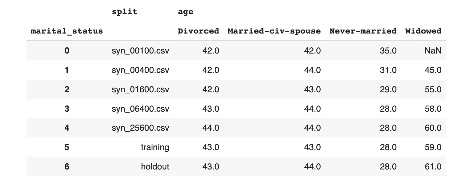
Then explore the age distribution, split by income:
sns.catplot(
    data=df_all,
    x='age',
    y='split',
    hue='income',
    kind='violin',
    split=True,
    legend=None
)
plt.legend(loc='upper right', title='', prop={'size': 8})
plt.show()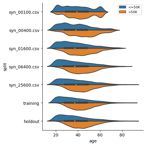
In both of these cases we see, again, that the synthetic datasets trained on more training samples resemble the original dataset more closely. We also see that the difference between the dataset trained on 6,400 samples and that trained on 25,600 seems to be minimal. This means that if the accuracy of these specific individual variable distributions is most important to you, you could confidently train your synthetic data generation model using just 6,400 samples (rather than the full 39,074 records). This will save you significantly in computational costs and runtime.
Rule Adherence
The original data has a 1:1 relationship between the education and education_num columns: each textual education level in the education column has a corresponding numerical value in the education_num column.
Let's check in how many cases the generated synthetic data has correctly retained that specific rule between these two columns.
First, display the matching columns in the original training data:
# display unique combinations of `education` and `education_num`
(df_trn[['education', 'education_num']]
 .drop_duplicates()
 .sort_values('education_num')
 .reset_index(drop=True)
)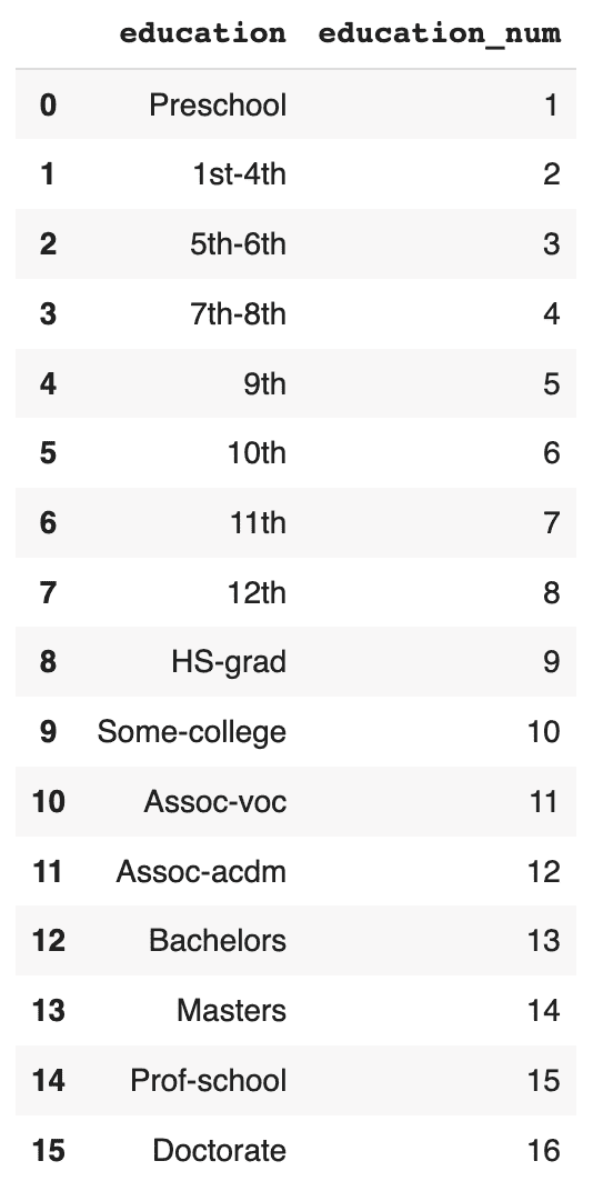
Now, convert the education column to Categorical dtype, sort and calculate the ratio of correct matches:
# convert `education` to Categorical with proper sort order
df['education'] = pd.Categorical(
    df['education'],
    categories=df_trn.sort_values('education_num')['education'].unique())

# calculate correct match
stats = (
    df.groupby('split')
    .apply(lambda x: (x['education'].cat.codes+1 == x['education_num']).mean())
)
stats = stats.to_frame('matches').reset_index()
stats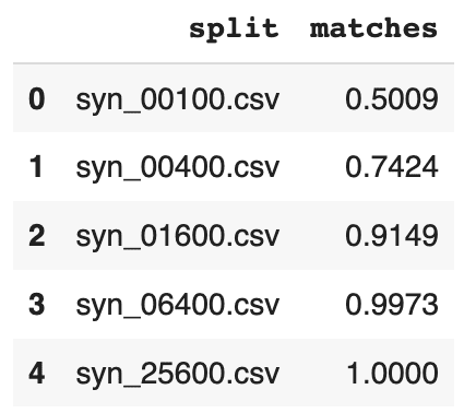
Visualize the results:
sns.catplot(
    data=stats,
    y='matches',
    x='split',
    kind='point',
    color='black'
)
plt.xticks(rotation=45)
plt.xlabel('')
plt.title('Share of Matches')
plt.show()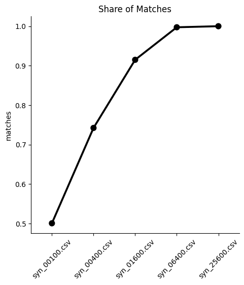
We can see from both the table and the plot that the dataset trained on just 100 samples severely underperforms, matching the right values in the columns only half of the time. While performance improves as the training samples increase, only the synthetic dataset generated using 25,600 samples is able to reproduce this rule adherence 100%. This means that if rule adherence for these columns is crucial to the quality of your synthetic data, you should probably opt for a training size of 25,600.
Downstream ML task
Finally, let’s evaluate the 5 synthetic datasets by evaluating their performance on a downstream machine learning task. This is also referred to as the Train-Synthetic-Test-Real evaluation methodology. You will train a ML model on each of the 5 synthetic datasets and then evaluate them on their performance against an actual holdout dataset containing real data which the ML model has never seen before (the remaining 20% of the dataset, which can be downloaded here).
The code block below defines the functions that will preprocess your data, train a LightGBM model and evaluate its performance. For more detailed descriptions of this code, take a look at the Train-Synthetic-Test-Real tutorial.
# import necessary libraries
import lightgbm as lgb
from lightgbm import early_stopping
from sklearn.model_selection import train_test_split
from sklearn.metrics import roc_auc_score

# define target column and value
target_col = 'income'
target_val = '>50K'

# prepare data, and split into features `X` and target `y`
def prepare_xy(df: pd.DataFrame):
    y = (df[target_col]==target_val).astype(int)
    str_cols = [
        col for col in df.select_dtypes(['object', 'string']).columns if col != target_col
    ]
    for col in str_cols:
        df[col] = pd.Categorical(df[col])
    cat_cols = [
        col for col in df.select_dtypes('category').columns if col != target_col
    ]
    num_cols = [
        col for col in df.select_dtypes('number').columns if col != target_col
    ]
    for col in num_cols:
        df[col] = df[col].astype('float')
    X = df[cat_cols + num_cols]
    return X, y


# train ML model with early stopping
def train_model(X, y):
    cat_cols = list(X.select_dtypes('category').columns)
    X_trn, X_val, y_trn, y_val = train_test_split(X, y, test_size=0.2, random_state=1)
    ds_trn = lgb.Dataset(
        X_trn,
        label=y_trn,
        categorical_feature=cat_cols,
        free_raw_data=False
    )
    ds_val = lgb.Dataset(
        X_val,
        label=y_val,
        categorical_feature=cat_cols,
        free_raw_data=False
    )
    model = lgb.train(
        params={
            'verbose': -1,
            'metric': 'auc',
            'objective': 'binary'
        },
        train_set=ds_trn,
        valid_sets=[ds_val],
        callbacks=[early_stopping(5)],
    )
    return model


# apply ML Model to some holdout data, report key metrics, and visualize scores
def evaluate_model(model, hol):
    X_hol, y_hol = prepare_xy(hol)
    probs = model.predict(X_hol)
    preds = (probs >= 0.5).astype(int)
    auc = roc_auc_score(y_hol, probs)
    return auc


def train_and_evaluate(df):
    X, y = prepare_xy(df)
    model = train_model(X, y)
    auc = evaluate_model(model, df_hol)
    return auc
Now calculate the performance metric for each of the 5 ML models:
aucs = {k: train_and_evaluate(df) for k, df in synthetic_datasets.items()}
aucs = pd.Series(aucs).round(3).to_frame('auc').reset_index()
And visualize the results:
sns.catplot(
    data=aucs,
    y='auc',
    x='index',
    kind='point',
    color='black'
)
plt.xticks(rotation=45)
plt.xlabel('')
plt.title('Predictive Performance (AUC) on Holdout')
plt.show()
We see, again, that optimal performance is achieved with the largest training sample size. Interestingly, the difference in performance between the dataset trained on 1,600 samples and the one trained on 6,400 samples is minimal in this case. This means that if your use case allows you to sacrifice a fraction of ML performance, you could train your synthetic data generator on just 1,600 samples and still get pretty great results.
In most cases, however, a 1% difference in ML accuracy is crucial to preserve and so most likely you would end up training on 25,600 samples. A worthwhile exercise here would be to train a synthetic generator using the full 39,074 training samples to see whether that performs even better.
Optimize your training sample size for synthetic data accuracy
In this tutorial you have seen first-hand the relationship between the size of your training samples and the resulting synthetic data quality. You have quantified and evaluated this relationship from multiple angles and with various use cases in mind, including looking at single variable distributions, rule adherence and ML utility. For the given dataset and the given synthesizer we can clearly observe an increase in synthetic data quality with a growing number of training samples across the board.
We have also observed that a holdout dataset will exhibit deviations from the training data due to sampling variance. With the holdout data being actual data that hasn't been seen before, it serves as a north star in terms of maximum achievable synthetic data accuracy. Read our blog post on benchmarking synthetic data generators for more on this topic.
What’s next?
In addition to walking through the above instructions, we suggest experimenting with the following in order to get an even better grasp of the relationship between training sample size and synthetic data accuracy:
- to limit model training to a few epochs, e.g. by setting the maximum number of epochs to 1 or 5 and study its impact on runtime and quality.
- to synthesize with different model_sizes: Small, Medium and Large, and study its impact on runtime and quality.
- to synthesize with the same settings several times to study the variability in quality across several runs.
- to calculate and compare your own statistics, and then compare the deviations between synthetic and training. The deviations between holdout and training can serve as a benchmark.
In this tutorial, you will learn how to validate synthetic data quality by evaluating its performance on a downstream Machine Learning (ML) task. The method you will learn is commonly referred to as the Train-Synthetic-Test-Real (TSTR) evaluation.
In a nutshell, we will train two ML models (one on original training data and one on synthetic data) and compare the performance of these two models in order to assess how well the synthetic data retains the statistical patterns present in the original data. The Python code for this tutorial is runnable and publicly available in this Google Colab notebook.
The TSTR evaluation serves as a robust measure of synthetic data quality because ML models rely on the accurate representation of deeper underlying patterns to perform effectively on previously unseen data. As a result, this approach offers a more reliable assessment than simply evaluating higher-level statistics.
The train-synthetic-test-real methodology
The TSTR method can be broken down into 5 steps:
- We start with an actual (real) data source and split this into a main dataset for training and a holdout dataset for evaluation.
- Next, we create a synthetic dataset only based on the training data.
- Then we train a Machine Learning (ML) model, and do so once using the synthetic data and once using the actual training data.
- We then evaluate the performance of each of these two models against the actual holdout data that was kept aside all along.
- By comparing the performance of these two models, we can assess how much utility has been retained by the synthesization method with respect to a specific ML task.
In the following sections, we will walk through each of these 5 steps using a real dataset and explain the Python code in detail.
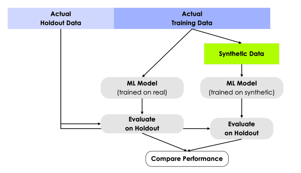
This testing framework simulates the real-world scenario in which a model is trained on historical data but has to perform in production on data it has never seen before. For this reason, it’s crucial to use a true holdout dataset for the evaluation in order to properly measure out-of-sample performance.
1. Data prep
We will be working with a pre-cleaned version of the UCI Adult Income dataset, which itself stems from the 1994 American Community Survey by the US census bureau. The dataset consists of 48,842 records, 14 mixed-type features and has 1 target variable, that indicates whether a respondent had or had not reported a high level of annual income. We will use this dataset because it's one of the go-to datasets to showcase machine learning models in action.
The following code snippet can be used to split a DataFrame into a training and a holdout dataset.
from sklearn.model_selection import train_test_split

df = pd.DataFrame({'x': range(10), 'y': range(10, 20)})
df_trn, df_hol = train_test_split(df, test_size=0.2, random_state=1)
display(df_trn)
display(df_hol)
In the repo accompanying this tutorial, the data has already been split for you to save you some precious time 🙂
- Download the training data census-training.csv by clicking here and pressing Ctrl+S or Cmd+S to save the file locally. This is an 80% sample of the full dataset. The remaining 20% sample can be fetched from here.
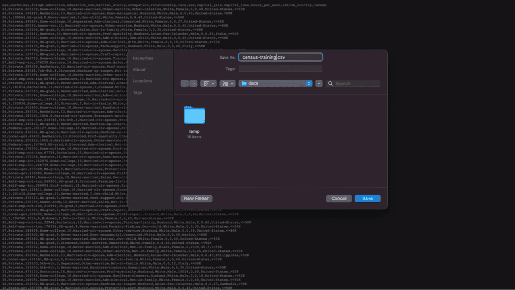
2. Data synthesis
Next, we will create the synthesized version of the training dataset. Synthesize census-training.csv via MOSTLY AI's synthetic data generator by following the steps outlined below. You can leave all settings at their default, and just proceed to launch the job.
- Navigate to “Synthetic Datasets”. Upload census-training.csv and click “Proceed”.
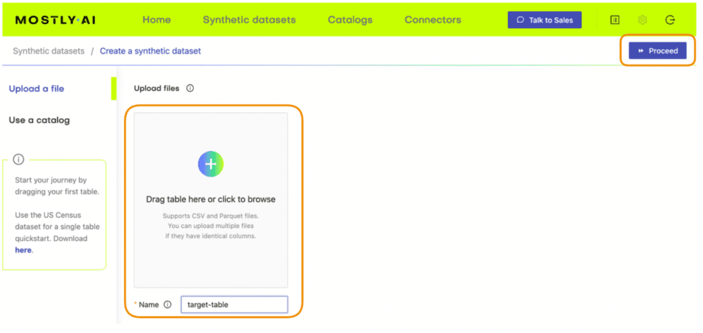
2. On the next page, click “Create a Synthetic Dataset” to launch the synthesization. You can leave all settings at their default.
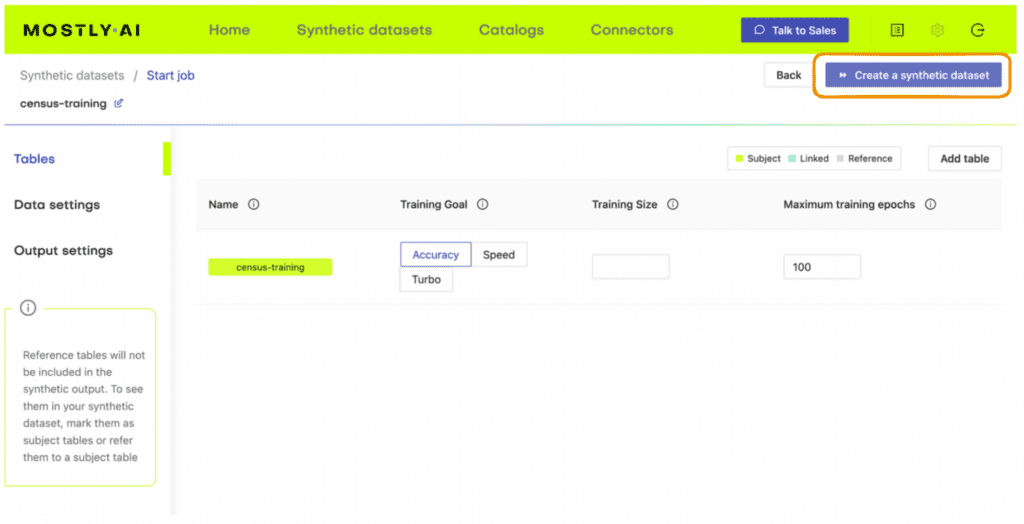
3. Follow the job’s progress using the UI and once the job has finished, download the generated synthetic data as CSV file to your computer. Optionally, you can also download a previously synthesized version here.
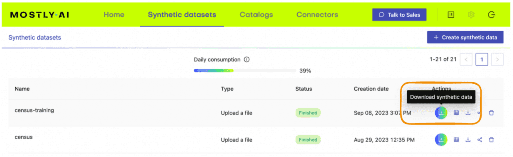
4. Return to your IDE or notebook and run the following code to create 3 DataFrames containing the training, synthesized and holdout data, respectively:
# upload synthetic dataset
import pandas as pd

try:
    # check whether we are in Google colab
    from google.colab import files
    print("running in COLAB mode")
    repo = 'https://github.com/mostly-ai/mostly-tutorials/raw/dev/train-synthetic-test-real'
    import io
    uploaded = files.upload()
    syn = pd.read_csv(io.BytesIO(list(uploaded.values())[0]))
    print(f"uploaded synthetic data with {syn.shape[0]:,} records and {syn.shape[1]:,} attributes")
except:
    print("running in LOCAL mode")
    repo = '.'
    print("adapt `syn_file_path` to point to your generated synthetic data file")
    syn_file_path = './census-synthetic.csv'
    syn = pd.read_csv(syn_file_path)
    print(f"read synthetic data with {syn.shape[0]:,} records and {syn.shape[1]:,} attributes")


# fetch training and holdout data
train = pd.read_csv(f'{repo}/census-training.csv')
print(f'fetched training data with {train.shape[0]:,} records and {train.shape[1]} attributes')
holdout = pd.read_csv(f'{repo}/census-holdout.csv')
print(f'fetched holdout data with {holdout.shape[0]:,} records and {holdout.shape[1]} attributes')
Before proceeding, let’s take a quick look at our freshly synthesized dataset by sampling 10 random records:
syn.sample(n=10)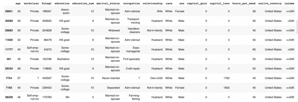
We can also get more specific by, for example, counting low-income and high-income records among the group of non-US citizens that have been divorced.
syn.loc[
    (syn["native_country"]!="United-States")
    & (syn["marital_status"]=="Divorced")
]['income'].value_counts()
<=50K 360
>50K 38
Name: income, dtype: int64Feel free to poke around the synthetic dataset more on your own to get a feel for the data.
3. ML training
Let's now train a state-of-the-art LightGBM classifier on top of the synthetic data, to then check how well it can predict whether an actual person reported an annual income of more than $50K or not. We will then compare the predictive accuracy to a model, that has been trained on the actual data, and see whether we were able to achieve a similar performance purely based on the synthetic data.
The following code block defines the target column and value and defines a function prepare_xy which preprocesses the data for ML training. The function casts the columns to the correct data types: columns containing strings are cast to categorical dtype and all numerical values are cast to float dtype. This is necessary for proper functioning of the LightGBM model. The function also splits the dataset into features X and target y.
Run the code block below to define the function.
# import necessary libraries
import lightgbm as lgb
from lightgbm import early_stopping
from sklearn.model_selection import train_test_split
from sklearn.metrics import roc_auc_score, accuracy_score
import seaborn as sns
import matplotlib.pyplot as plt

# define target column and value
target_col = 'income'
target_val = '>50K'

# define preprocessing function
def prepare_xy(df):
    y = (df[target_col]==target_val).astype(int)
    str_cols = [
        col for col in df.select_dtypes(['object', 'string'])
        .columns if col != target_col
    ]
    for col in str_cols:
        df[col] = pd.Categorical(df[col])
    cat_cols = [col for col in df.select_dtypes('category').columns if col != target_col]
    num_cols = [col for col in df.select_dtypes('number').columns if col != target_col]
    for col in num_cols:
        df[col] = df[col].astype('float')
    X = df[cat_cols + num_cols]
    return X, y
Now run the function prepare_xy to preprocess the data:
X_syn, y_syn = prepare_xy(syn)Next, we define a function train_model which will execute the ML training. The dataset is split into training and evaluation splits and the model is trained on the training dataset using some well-established base parameters. We specify early_stopping after 5 rounds without performance improvement in order to prevent overfitting.
3. Run the code block below to define the training function:
def train_model(X, y):
    cat_cols = list(X.select_dtypes('category').columns)
    X_trn, X_val, y_trn, y_val = train_test_split(X, y, test_size=0.2, random_state=1)
    ds_trn = lgb.Dataset(
        X_trn,
        label=y_trn,
        categorical_feature=cat_cols,
        free_raw_data=False
    )
    ds_val = lgb.Dataset(
        X_val,
        label=y_val,
        categorical_feature=cat_cols,
        free_raw_data=False
    )
    model = lgb.train(
        params={
            'verbose': -1,
            'metric': 'auc',
            'objective': 'binary'
        },
        train_set=ds_trn,
        valid_sets=[ds_val],
        callbacks=[early_stopping(5)],
    )
    return model
4. Now execute the training function:
model_syn = train_model(X_syn, y_syn)4. Synthetic data quality evaluation with ML
The next step is to evaluate the model’s performance on predicting the target feature y, which is whether or not a respondent had a high income. In this step we will be using the holdout dataset (which the model has never seen before) to evaluate the performance of the model trained on synthetic data: Train Synthetic, Test Real.
We’ll use two performance metrics:
- Accuracy: This is the probability to correctly predict the income class of a randomly selected record.
- AUC (Area-Under-Curve): This is the probability to correctly predict the income class, if two records, one of high-income and one of low-income are given.
Whereas the accuracy informs about the overall ability to get the class attribution correct, the AUC specifically informs about the ability to properly rank records, with respect to their probability of being within the target class or not. In both cases, the higher the metric, the better the predictive accuracy of the model.
We define a function evaluate_model which will perform the evaluation. This function first preprocesses the holdout data and then uses the model we have just trained on our synthetic data to try to predict the holdout dataset.
- Run the code block below to define the evaluation function:
def evaluate_model(model, hol):
    X_hol, y_hol = prepare_xy(hol)
    probs = model.predict(X_hol)
    preds = (probs >= 0.5).astype(int)
    auc = roc_auc_score(y_hol, probs)
    acc = accuracy_score(y_hol, preds)
    probs_df = pd.concat([
        pd.Series(probs, name='probability').reset_index(drop=True),
        pd.Series(y_hol, name=target_col).reset_index(drop=True)
    ], axis=1)
    sns.displot(
        data=probs_df,
        x='probability',
        hue=target_col,
        bins=20,
        multiple="stack"
    )
    plt.title(f"Accuracy: {acc:.1%}, AUC: {auc:.1%}", fontsize=20)
    plt.show()
    return auc
2. Now run the evaluation function:
auc_syn = evaluate_model(model_syn, holdout)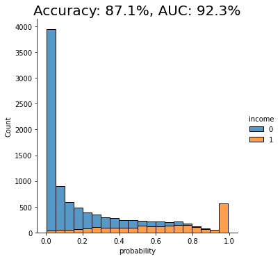
The displayed chart shows the distribution of scores that the model assigned to each of the holdout records. A score close to 0 means that model is very confident that the record is of low income. A score close to 1 means that the model is very confident that it's a high income record. These scores are further split by their actual outcome, i.e. whether they are or are not actually high income. This allows us to visually inspect the model's confidence in assigning the right scores.
We can see that the model trained on synthetic data seems to perform quite well when testing against real data it has never seen before (i.e. the holdout dataset). Both the accuracy and AUC scores give us confidence that this model may perform well in production.
But the real test is: how does the performance of this model trained on synthetic data compare against the performance of a model trained on real data? Remember: the purpose of this exercise is to discover whether we can use high-quality synthetic data to train our ML models instead of the original data (to protect data privacy) without losing significant predictive performance.
5. ML performance comparison
So let's now compare the results achieved on synthetic data with a model trained on real data. For a very good synthesizer, we expect to see a predictive performance of the two models being close to each other.
- Run the same 3 functions as we did above to prepare the data, train the model and evaluate it, but this time using the original dataset rather than the synthetic data:
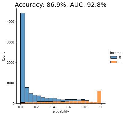
For the given dataset, and the given synthesizer, we can observe a near on-par performance of the synthetic data with respect to the given downstream ML task. Both accuracy scores are around 87% and both AUC scores are around 92%, with a maximum of 0.5% difference.
This means that in this case you can train your LightGBM machine learning model purely on synthetic data and be confident that it will yield equally performant results as if it were trained on real data, but without ever putting the privacy of any of the contained individuals at any risk.
What did we learn about synthetic data quality evaluations?
This tutorial has introduced you to the Train Synthetic Test Real methodology for synthetic data quality evaluations, specifically by measuring its utility on a downstream ML task. This evaluation method is more robust than only looking at high-level statistics because ML models rely on the accurate representation of deeper underlying patterns to perform effectively on previously unseen data.
By testing your model trained on synthetic data on a holdout dataset containing original (real) data that the model has never seen before, you can now effectively assess the quality of your synthesized datasets. With the right dataset, model and synthesizer, you can train your ML models entirely on synthetic data and be confident that you are getting maximum predictive power and privacy preservation.
What’s next?
In addition to walking through the above instructions, we suggest:
- to run the Train-Synthetic-Test-Real synthetic data quality evaluation
- using a different dataset, eg. the UCI bank-marketing dataset
- using a different downstream ML model, eg. a RandomForest model
- using a different synthesizer, eg. SynthCity, SDV, etc.
- to check the impact of synthetic upsampling by generating 10x or 100x the original data records, and see whether it improves ML accuracy.
- What is data migration?
- How to do data migration with synthetic data?
- Challenges in data migration
- The role and benefits of synthetic data generation in data migration
- Real-world use cases and scenarios
- Real data migration vs synthetic data migration
- How to do data migration? Use synthetic data!
What is data migration, and how to do it well
Data migration is a critical process in data management and technology. Whether it involves upgrading systems, transitioning to the cloud, or consolidating databases, data migration is an integral part of keeping an organization's data infrastructure up-to-date and efficient.
However, data migration comes with its own set of challenges. Ensuring data integrity, preserving data privacy, and validating the accuracy of transferred data are among the primary concerns of data professionals. This is where synthetic data steps in as a powerful and innovative solution.
Synthetic data is artificial data that mimics the characteristics of real data without containing any actual information about individuals or entities. It's generated through mathematical models, algorithms, or statistical techniques. In the context of data migration projects, synthetic data serves as a solution, offering a host of benefits that address the challenges associated with traditional data migration.
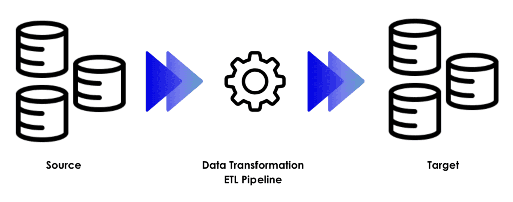
How to do data migration with synthetic data
So, why is synthetic data relevant in the context of data migration projects?
Imagine this scenario: You're tasked with migrating a massive customer database from one system to another. The data contains sensitive information like names, addresses, and purchase histories. It is critical to ensure data privacy and security. You must also extensively test your migration process to avoid data damage, loss, or format discrepancies. Furthermore, the enormous amount of data makes testing difficult and time-consuming.
This is precisely where AI-generated synthetic data shines. It allows you to create data that looks, feels, and behaves like the real thing, without exposing sensitive information. Synthetic data provides a controlled and secure environment for testing, ensuring that the migration process works seamlessly while safeguarding privacy and security.
In the following sections, we'll explore in detail how synthetic data addresses these challenges and offers a pathway to smoother, more efficient, and privacy-conscious data migration. We'll discuss its benefits, use cases, best practices, and more, so you can leverage the power of synthetic data to enhance your data migration projects.
Challenges in data migration
Data migration is a multifaceted process that, while necessary, often presents several challenges and complexities. These challenges can vary depending on the scale, scope, and nature of the migration project.
- Data Format Discrepancies: One of the most difficult aspects of data migration is dealing with data format discrepancies between the source and target systems. These distinctions can include differences in data architecture, data formats, and encoding standards. It is a difficult process to migrate data while verifying that it complies with the new format.
- Data Cleansing and Quality Assurance: Data quality concerns are widespread, and they may worsen during data transfer. Data that is inaccurate, incomplete, or duplicate might cause mistakes and inconsistencies in the target system. Cleaning and verifying data to ensure it meets quality requirements takes time and attention to detail.
- Data Volume and Scale: Large data migrations may strain resources and infrastructure. To prevent performance bottlenecks, data migration initiatives must be prepared to handle huge datasets efficiently. This frequently necessitates meticulous planning and optimization.
- Data Mapping and Transformation: Data is frequently mapped and converted to meet the requirements of the target system. This entails developing rules and logic for data conversion, which can be complex and error-prone if not handled methodically.
- Data Privacy and Security: It is critical to safeguard sensitive data during relocation. It is difficult to ensure that sensitive information is not exposed or compromised, especially when dealing with legislation such as GDPR or HIPAA.
- Testing and Validation: Testing and validation are required to ensure that the migration process is error-free and that the data in the target system appropriately replicates the source data. This entails writing test cases and ensuring that they cover a wide range of situations and edge scenarios.
Organizations frequently seek new ways to expedite the data migration process in consideration of these challenges. One such solution is the integration of synthetic data using MOSTLY AI’s synthetic data generator, which can significantly mitigate many of these challenges by providing a controlled, secure, and privacy-conscious environment for testing and validation without exposing sensitive information. If this piques your interest, please read on to understand how MOSTLY AI addresses these challenges and contributes to successful data migration projects.
The role and benefits of synthetic data generation in data migration
As explained above, data migration often involves transferring data from one system to another, and these systems may have different data formats, structures, and schemas. These format disparities can pose significant challenges, as data from the source system may not align neatly with the requirements of the target system.
Synthetic data generation excels in the task of harmonizing data formats by being adaptable and customizable. Synthetic data generators like MOSTLY AI, are designed to replicate the structure and format of the target system. This means that when you generate synthetic data for testing, it can match the schema and format specifications of the system you're migrating data to. When you test the migration process using synthetic data that matches the target system's format, you reduce the risk of errors and unexpected issues during the actual migration. This alignment ensures a smoother transition, as data is more likely to fit seamlessly into the new system without the need for complex data transformations or extensive manual adjustments.
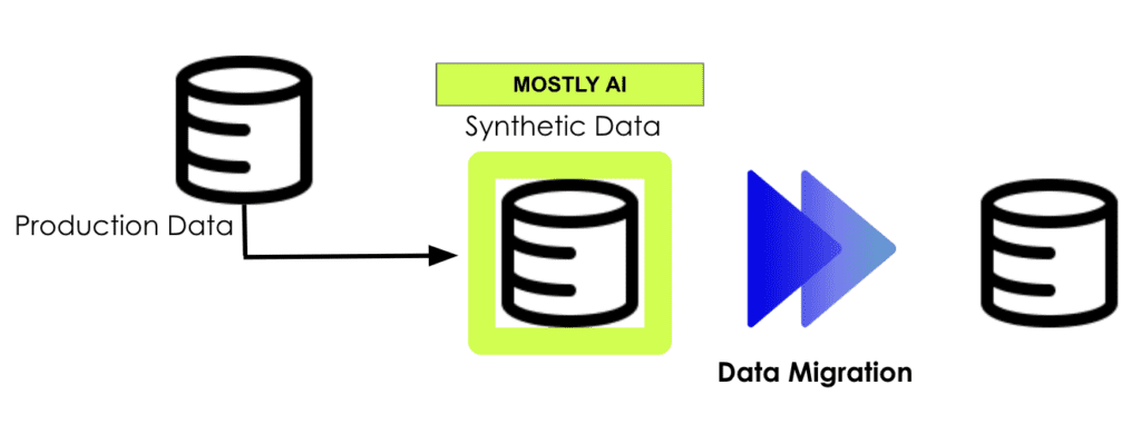
Data professionals during their data migration journey, can realise that synthetic data generated by MOSTLY AI plays a crucial role in maintaining data integrity and streamlining testing processes. Data integrity is protected via synthetic data. Its well-defined characteristics make any inconsistencies or errors during migration immediately noticeable. This allows for quick identification and resolution of issues, ensuring the accuracy and reliability of the migrated data.
On top of that, synthetic data simplifies the testing of data mapping and transformation rules. Organizations can create diverse test scenarios that encompass various mapping and transformation scenarios. This approach ensures comprehensive testing and validation, reducing the risk of errors in the migration process.
Synthetic data stands as a solution for organizations seeking to maintain data privacy and security during testing and validation. Its artificial nature, compliance with privacy regulations, high level of security, and customization options make it an ideal choice, especially in scenarios where real-world sensitive information must be shielded from exposure and potential breaches. MOSTLY AI is a well-known solution for protecting personally identifiable information (PII), maintaining data privacy and security of your original data.
Real-world use cases and scenarios
Data migration in insurance
Scenario: An insurance company is migrating policyholder data from legacy systems to a modern platform to enhance customer service and streamline operations.
Use of Synthetic Data: Synthetic policyholder profiles can be generated to replicate real policy data, including policy types, coverage details, and claims history. This synthetic data allows thorough testing of the migration process, ensuring data accuracy, privacy compliance, and adherence to insurance industry regulations.
Data migration in healthcare
Scenario: A healthcare provider is transitioning to a new electronic health record (EHR) system, necessitating the transfer of patient medical records.
Use of Synthetic Data: Synthetic patient records can be created to simulate real EHRs, preserving patient privacy and complying with strict healthcare regulations like HIPAA. These synthetic records enable comprehensive testing and validation of the EHR migration process, including data mapping and access control.
Data migration in financial services and banking
Scenario: A financial institution is merging with another bank, requiring the consolidation of customer accounts, transaction histories, and investment portfolios.
Use of Synthetic Data: Synthetic customer profiles and financial transactions can be generated to replicate real banking data. This synthetic data facilitates rigorous testing and validation of the migration, ensuring data accuracy, compliance with financial regulations, and the security of sensitive financial information.
Real data migration vs synthetic data migration
| Differences | Real Data Migration | Synthetic Data Migration |
| Data Privacy and Compliance | Using real data in testing poses privacy risks, requiring extensive measures to anonymize or pseudonymize sensitive information. Compliance can be challenging to maintain. | Synthetic data is artificial and does not contain real-world information, making it ideal for testing without privacy concerns. It ensures compliance with data protection regulations. |
| Data Security | Handling real data in testing can expose sensitive information to security risks, necessitating stringent security measures. | Synthetic data is generated in controlled environments and is devoid of real-world vulnerabilities, making it highly secure. |
| Testing Scenarios | Testing with real data may be limited by the availability of specific scenarios or edge cases, potentially leaving gaps in validation. | Synthetic data allows for the creation of diverse and extreme testing scenarios, ensuring comprehensive validation of migration processes. |
| Scalability | Testing with massive datasets can be resource-intensive and challenging to manage. | Synthetic data can be generated at any scale, making it suitable for testing large-scale migrations. |
| Flexibility | Real data may require complex transformations to align with the target system, increasing the risk of errors. | Synthetic data can be customized to match target system formats, facilitating format harmonization. |
How do you do data migration? Use synthetic data!
In the world of data migration, synthetic data from MOSTLY AI emerges as the game-changing solution. It simplifies processes, enhances privacy, and ensures data accuracy in sectors like insurance, healthcare, and finance.
Explore MOSTLY AI's synthetic data generator for seamless data migration. Discover how synthetic data can boost your organization's data migration projects while ensuring data privacy and compliance.
This article explains what data drift is, how it affects machine learning models in production, what the difference between data drift and concept drift is, and what you can do to tackle data drift using synthetic data.
What is data drift?
“Data drift” is a term in machine learning that refers to the phenomenon in which a machine learning model’s performance slowly decreases over time. This happens because machine learning models are trained on historical data (i.e. “the past”) but then use current data (i.e. “the present”) when they are being used in production. In reality, the historical data and the current data may have different statistical characteristics and this is what we call “data drift”: the data used for predictions starts to drift from the data used for training. This means the machine learning model is no longer fully optimized for the data it is seeing.
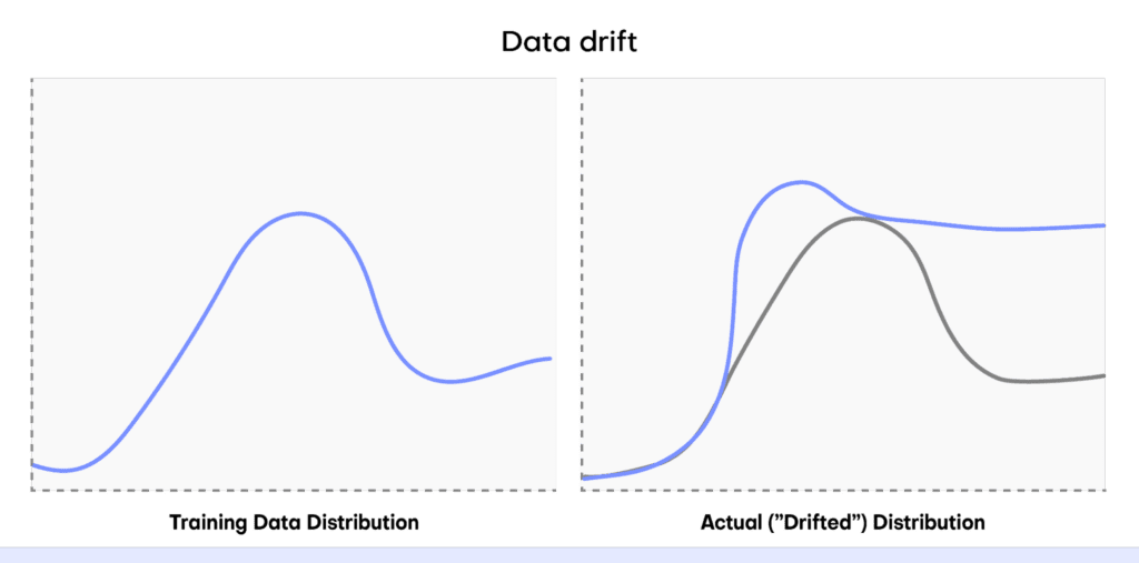
How does data drift affect ML models?
Drift can be a big problem when using machine learning models in the real world, causing a decrease in predictive power. For example, let’s say we have trained a machine learning model to accurately predict the quarterly sales of a particular fashion brand. We then put this model into production.
At first it operates well: the actual data it is receiving (from the present) resembles the data that was used to train the model (from the past). But then something unexpected happens. A popular influencer spontaneously posts about the fashion brand and the post goes viral. Sales sky-rocket in a way that the machine learning model could never have foreseen because nothing like the unexpected viral post event was present in the training data.
This causes a significant change in the statistical distribution of the input data (i.e. “data drift”) and the machine learning model no longer performs at optimum performance. The model loses accuracy and may even produce unreliable predictions if the data distributions vary significantly.
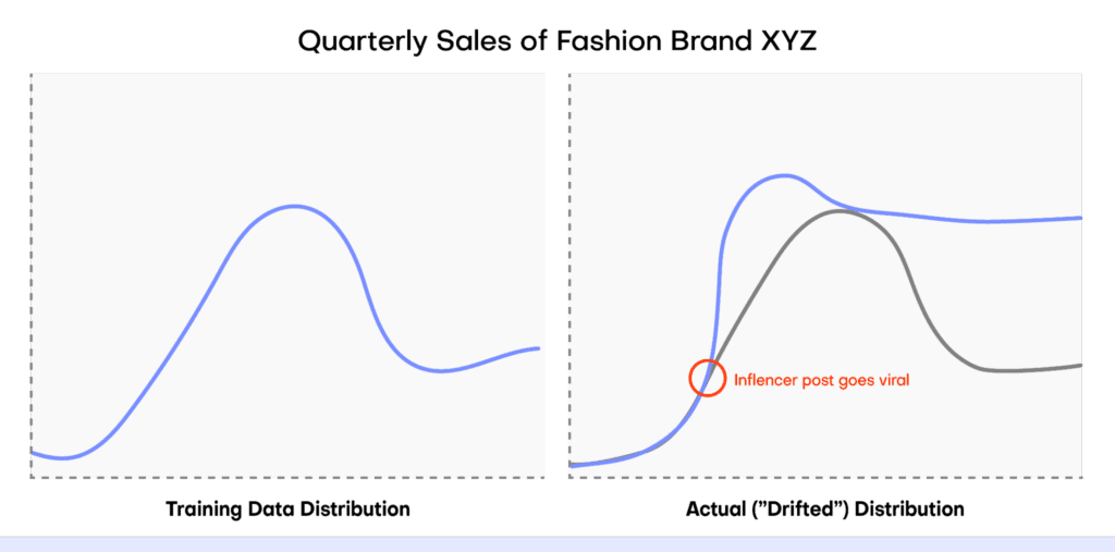
Data drift vs concept drift
There are different kinds of drift that can be observed in machine learning projects. Data drift refers specifically to the phenomenon in which the distribution of the real-world data used when the model is in production drifts from the data that was used for training.
Concept drift refers to the situation in which the relationship between features in the data changes over time. In this case, the pattern (or “concept”) that the machine learning model is trying to learn is evolving. In short, data drift deals with changes in the data that the model uses to make predictions, whereas concept drift refers to changes in the patterns between features in the data.
How can I deal with data drift?
Data drift is a complex phenomenon that generally requires a multidimensional approach to solve. Some of the most effective things you can do to deal with data drift include:
- Retrain your machine learning model on fresh data that includes the drifted distribution so that the model is performing at peak performance again.
- Perform robust feature engineering so that features are less sensitive to changes in the underlying data.
- Use ensemble methods like model blending and stacking or building a fully-online machine learning pipeline that can continuously update and retrain itself as new data comes in.
In practice, retraining a machine learning model with fresh data is one of the most common methods used to deal with data drift. However, this approach comes with some drawbacks. Acquiring new data that is ready for training a machine learning model is often:
- Expensive and time-consuming;
- Disruptive to ongoing workflows and processes;
- Difficult to execute because of privacy regulations.
Tackle data drift with synthetic data
Synthetic data generation can help you tackle data drift by providing a high-quality, low-friction source of data on which you can retrain your machine learning models. Synthetic data generators enable you to produce virtually limitless data and often give you fine-grained control over the distributions of this new data. By accurately modeling new synthetic datasets, you can then update your machine learning model to incorporate the drifted data distribution.
We’ve broken it down into 5 steps for clarity:
- Detect your data drift
- Understand your data drift
- Generate synthetic data
- Retrain your model
- Monitor and repeat
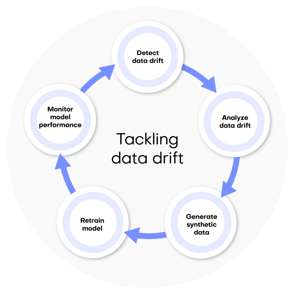
1. Detect your data drift
Detecting data drift should be a fundamental part of any machine learning life cycle. There are many ways to perform data drift detection and many resources to learn about it. This article focuses on solutions that will help you fix data drift once it has been detected.
2. Understand your data drift
Before tackling data drift, it’s important that you have a good understanding of its nature and potential causes. Analyze your model and the incoming data to identify points where the data is drifting and analyze its statistical characteristics. This will help you understand how to incorporate the data drift into your updated model.
For example, in the case of the quarterly fashion sales predictions mentioned above, the fact that we can reliably trace the data drift to the viral influencer post helps us know how to deal with the data drift. It’s reasonable to expect the influencer post to have lasting effects on the fashion brand’s perception and future sales: we should therefore adjust our data projections to include some of the ripple effects of this unexpected sales boost.
On the contrary, if we had instead seen a massive but temporary drop in sales due to a failure in the webshop’s main server, we may want to choose not to incorporate this data at all in the projections for next quarter, the assumption here being that the webshop will not experience another failure.
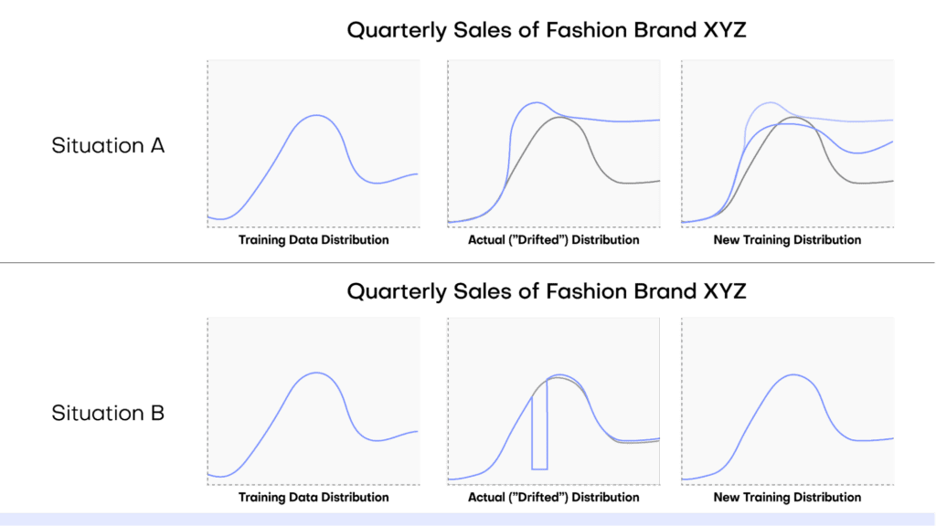
3. Generate synthetic data
Once you have a good understanding of the statistical nature and potential sources of your data drift, you can then proceed to use synthetic data generation to supplement your training dataset with cases that might occur due to data drift.
We’ll walk through how to generate the right kind of synthetic data to tackle your data drift with MOSTLY AI's synthetic data platform, using a technique called conditional generation.
- Split your dataset into two separate tables: one table containing the ID column and the columns containing your desired target features, and a second table containing the ID column along with all of the other predictor columns.
- Log in to your MOSTLY AI account.
- Launch a new job using the “Create Synthetic Data” button in the “Synthetic Datasets” tab. Upload the first table (containing the ID column and the target feature(s) to start a new job and then add the second table.
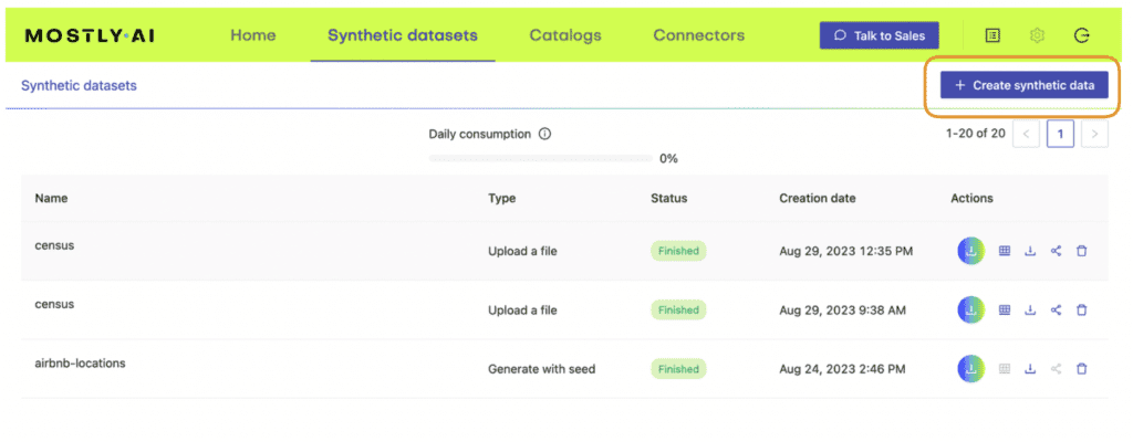
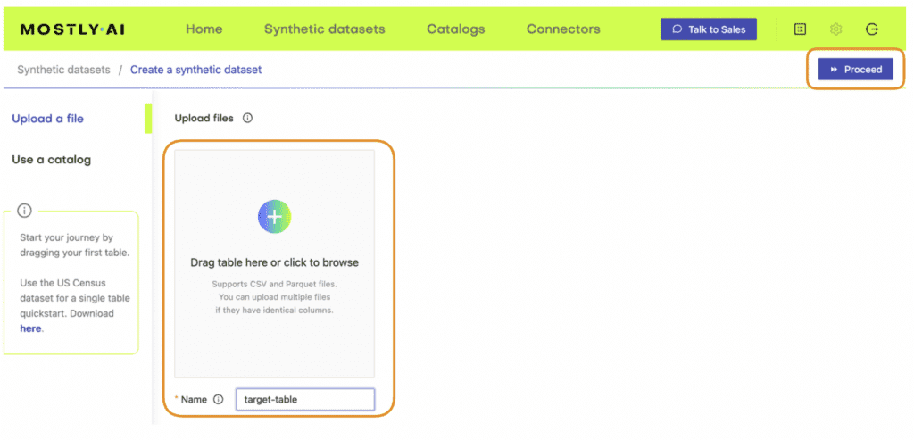
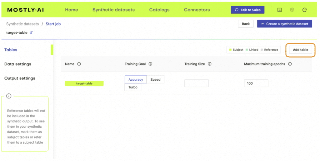
4. Define the relationship between the two tables using the Data Settings tab and navigating to the settings for the table containing the predictor columns. Click on the gear icon to the right of the ID column and set the following settings:
Generation Method: Foreign Key
Foreign Key: Type: Context
Parent Table: <your-table-with-target-column>
Parent Primary column: <id-column-of-target-table>
Save the settings. Under the “Tables” tab you should now see that the predictor table has changed into a Linked Table (lime green color coding).
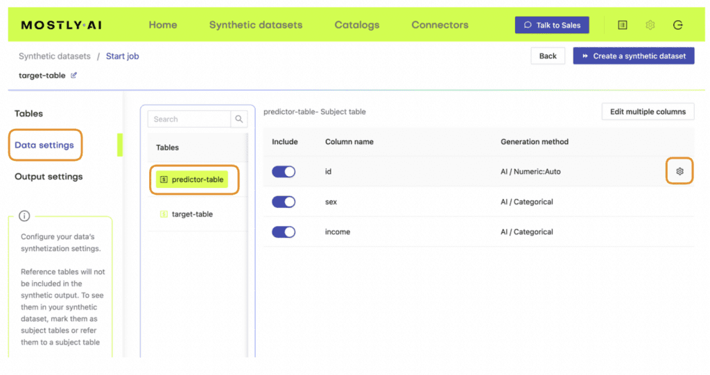
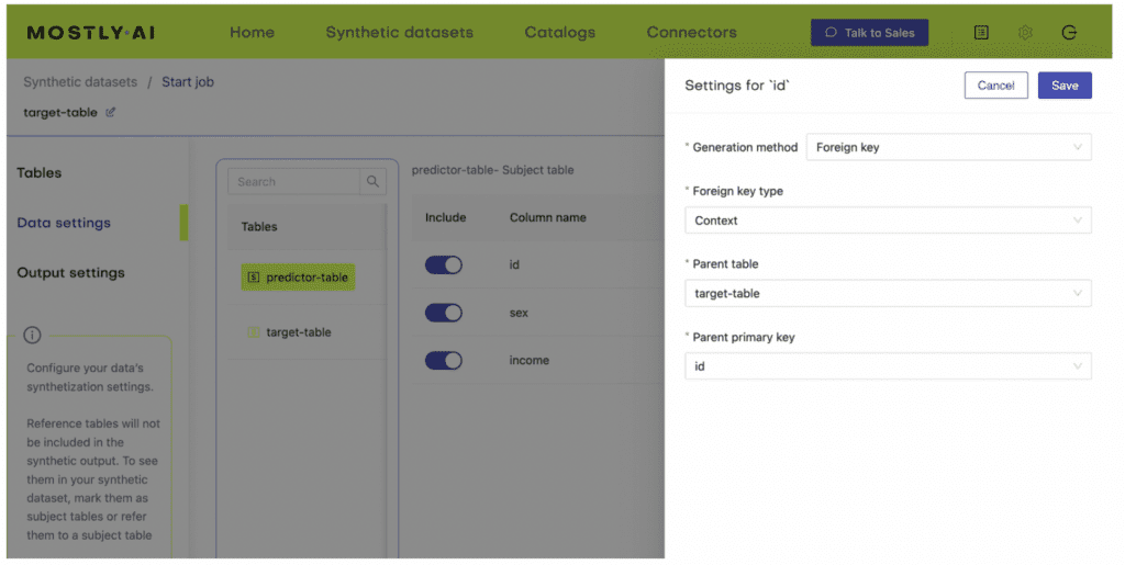
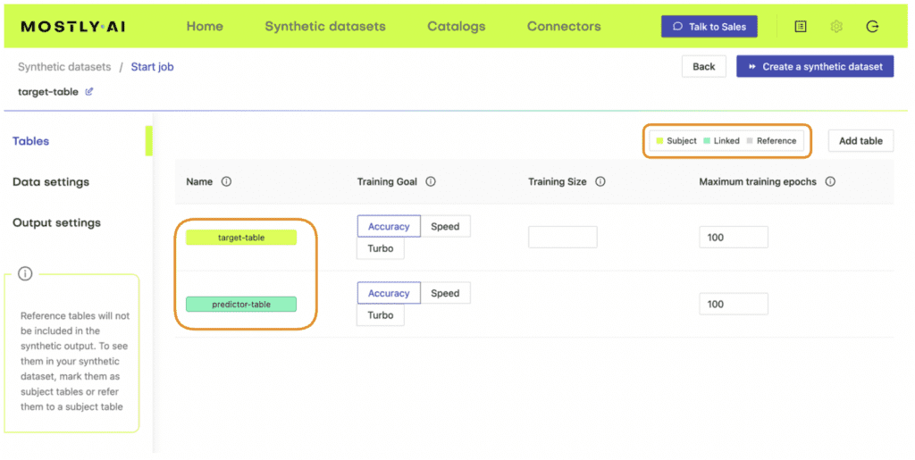
5. Once the job has been completed, select the “Generate more data” action on the right-hand side of the newly-generated dataset row and select “Generate with seed” to perform conditional generation.
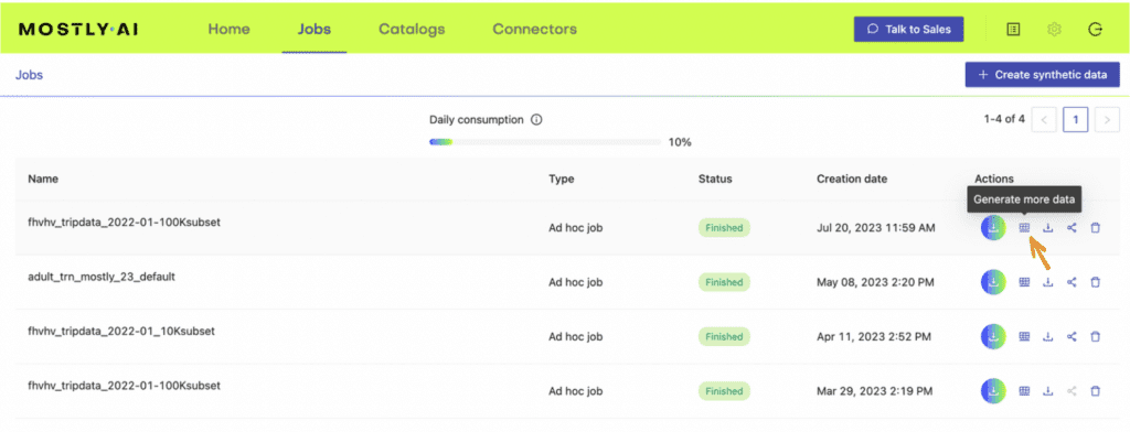
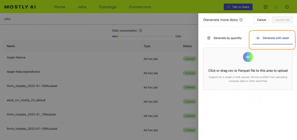
6. Now upload a subject table with a different kind of distribution.
This subject table can be generated manually or programmatically and should contain the drifted distribution. The simulated subject table (containing the drifted target feature distribution) will be used to generate a synthetic dataset (i.e. the predictor columns) that would produce the new, drifted distribution.
In our viral fashion post example, we would create a simulation of the target feature (sales) that follows the “new training distribution” depicted in Figure 4 above and use this to generate a synthetic dataset.
Open-source Python packages like NumPy or SciPy enable you to perform fine-grained data simulation. You can use MOSTLY AI’s rebalancing feature to programmatically simulate drifted target feature distributions for categorical columns.
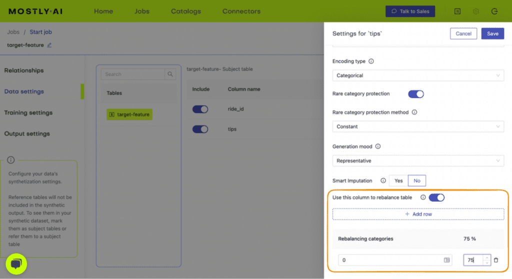
7. Repeat for all the different scenarios you want to model.
To properly accommodate all of the possible future scenarios, you may want to create multiple simulated datasets, each with a different assumption and associated distribution. In the case of our viral fashion post, we may want to create three simulations: one in which sales continue to skyrocket at the same rate as we saw this quarter, one in which sales just go back to ‘normal’ (i.e. the influencer post has no lasting effect), and a third scenario that takes the average of these two extremes. With these 3 synthetic datasets we can then train different models to predict 3 kinds of possible future scenarios.
4. Re-train your model
With your freshly generated synthetic data ready, you can now proceed to re-train your machine learning model. You can use just the synthetic data or a mix of real and synthetic data, depending on the privacy requirements of your model.
5. Monitor model performance and repeat
Finally, make sure to put precise monitoring tools in place to continue to detect data drift. For example, you could use open-source Python libraries like Evidently or NannyML to keep track of your model performance throughout the machine learning lifecycle. When your model metrics indicate a recurrence of data drift, update your synthetic data to reflect the new distributions and re-train your model.
Tackling data drift with MOSTLY AI
Synthetic data generation can help you tackle data drift by making it easy to simulate potential future scenarios based on new statistical distributions of the data. By providing a high-quality, low-friction source of data on which you can retrain your machine learning models, synthetic data generators enable you to produce virtually limitless data to model changes in the underlying data. MOSTLY AI gives you fine-grained control over the distributions of this new data so you can accurately model new synthetic datasets that take into consideration the drifted data distributions.
Try it out today – the first 100K rows of synthetic data are on us!
There is something different about Merkur Versicherung AG. It’s the oldest insurance company in Austria, but it doesn’t feel like it.
For starters, there’s the Campus HQ in Graz. An Illuminous race track lines the floor of the open plan space. The vibrant lobby is filled with eclectic artwork and unconventional furniture. And there’s a beautiful coffee dock beside the fully functioning gym in the lobby.
Then, there’s the people. One team in particular stands out amongst the crowd: the Merkur Innovation Lab. A group of self professed “geeks, data wizards, future makers” with some “insurance guys” thrown in for good measure. Insurance innovation is born right here. Daniela Pak-Graf, the managing director of Merkur Innovation Lab — the innovation arm of Merkur Insurance, told us in the Data Democratization Podcast:
“Merkur Innovation Lab is the small daughter, the small startup of a very old company. Our CEO had the idea, we have so much data, and we're using the data only for calculating insurance products, calculating our costs, and in the era of big data of Google, of Amazon, Netflix, there have to be more possibilities for health insurance data too. He said, "Yes, a new project, a new business, what can we do with our data?" Since 2020, we are doing a lot.”
Oh, and then there’s synthetic health data.
The Merkur Innovation Lab has fast become a blueprint for other organizations looking to develop insurance innovations by adopting synthetic data. In the following, we’ll introduce three insurance innovations powered by synthetic data adoption.
Insurance innovation no. 1: data democratization
Problem
Like many other data-driven teams, the Merkur Innovation Lab team faced the challenge of ensuring data privacy while still benefiting from valuable insights. The team experimented with data anonymization and aggregation but realized that it fell short of providing complete protection. The search for a more comprehensive solution led them to the world of synthetic data.
Solution
According to Daniela Pak-Graf, the solution to the problem is synthetic data:
"We found our way around it, and we are innovating with the most sensitive data there is, health data. Thanks to MOSTLY."
Merkur didn’t waste time in leveraging the power of synthetic data to quickly unlock the insights contained within their sensitive customer data. The team has created a beautifully integrated and automated data pipeline that enables systematic synthetic data generation on a daily basis, fueling insurance innovations across the organization. Here’s how they crafted their synthetic data pipeline:
- All “active customer” data (=600k rows, 55 columns) is extracted from a source Oracle database
- That original data is uploaded to MOSTLY AI’s synthetic data platform via a data catalog tool
- The synthesization process is triggered by a REST API
- Apache Airflow then writes the output synthetic data to the destination PostgreSQL database
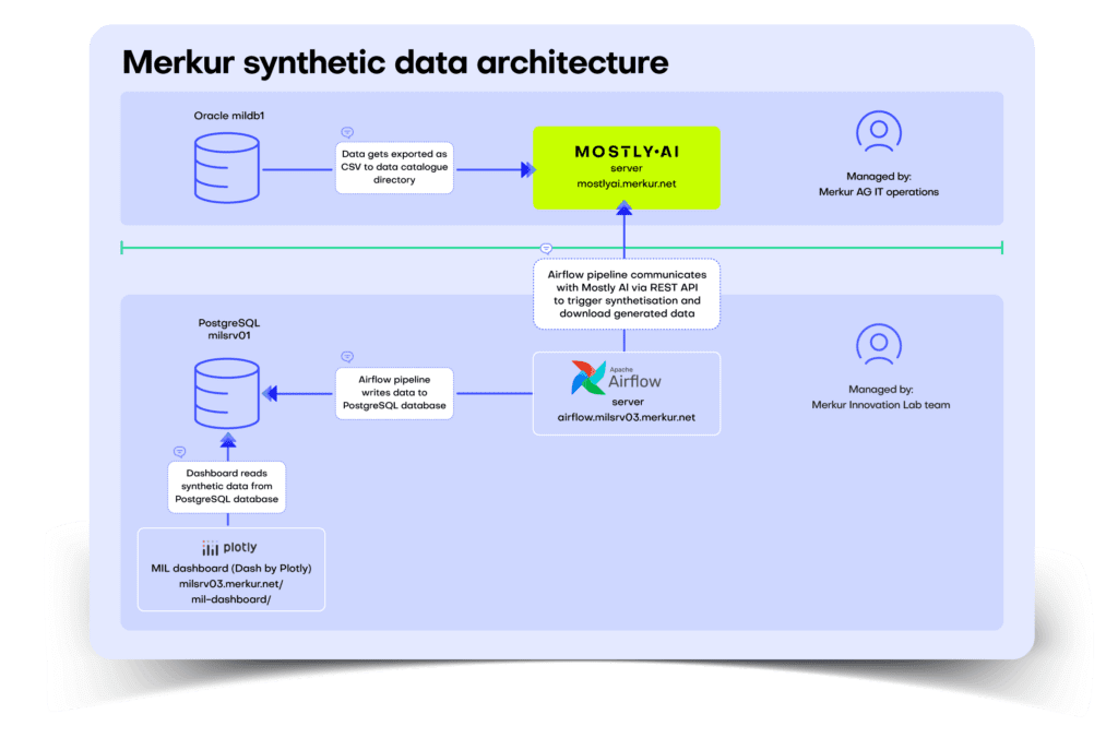
Proof
The end-to-end automated workflow has cut Merkur’s time-to-data from 1-month, to 1-day. The resulting synthetic granular health data is read into a dynamic dashboard to showcase a tailored ‘Monetary Analysis’ of Merkur’s customer population. And the data is available for consumption by anyone at any time. True data democratization and insurance innovation on the tap.
Insurance innovation no. 2: external data sharing
Problem
As we know, traditional data sharing approaches, particularly in sensitive industries like health and finance, often faced complexity due to regulatory constraints and privacy concerns. Synthetic data offered a quick and secure solution to facilitate data collaboration, without which scaling insurance innovations would be impossible.
Solution
According to Daniela:
“...one of the biggest opportunities is working with third parties. When speaking to other companies, not only insurance companies, but companies working with health data or customer data, there's always the problem, "How can we work together?" There are quite complex algorithms. I don't know, homomorphic encryption. No one understands homomorphic encryption, and it's not something which can be done quickly. Using synthetic data, it's a quick fix if you have a dedicated team who can work with synthetic data.”
Proof
One exciting collaboration enabled by synthetic data is Merkur Innovation Lab’s work with Stryker Labs. Stryker Labs is a startup focused on providing training management tools for professional athletes. The collaboration aims to extend the benefits of proactive healthcare and injury prevention to all enthusiasts and hobby athletes by merging diverse datasets from the adjacent worlds of sport and health. Daniela explained the concept:
“The idea is to use their expertise and our knowledge about injuries, the results, the medication, how long with which injury you have to stay in hospital, what's the prescribed rehabilitation, and so on. The idea is to use their business idea, our business idea, and develop a new one where the prevention of injuries is not only for professional sports, but also for you, me, the occasional runner, the occasional tennis player, the occasional, I don't know.”
This exciting venture has the potential to improve the well-being of a broader and more diverse population, beyond the privileged few who make it into the professional sporting ranks.
Insurance innovation no. 3: empowering women in healthcare
Another promising aspect of synthetic data lies in its potential to address gender bias and promote fairness in healthcare. By including a more diverse dataset, synthetic data can pave the way for personalized, fairer health services for women. In the future, Merkur Innovation Lab plans to leverage synthetic data to develop predictive models and medication tailored for women; it marks a step towards achieving better healthcare equality. According to Daniela:
“...it could be a solution to doing machine learning, developing machine learning algorithms with less bias. I don't know, minorities, gender equality. We are now trying to do a few POCs. How to use synthetic data for more ethical algorithms and less biased algorithms.”
The insurance industry and innovation
Insurance companies have always been amongst the most data-savvy innovators. Looking ahead, we predict that the insurance sector will continue to lead the way in adopting sophisticated AI and analytics. The list of AI use cases in insurance continues to grow and with it, the need for fast and privacy safe data access. Synthetic data in insurance unlocks the vast amount of intelligence locked up in customer data in a safe and privacy-compliant way. Synthetic healthcare data platforms are becoming a focal point for companies looking to accelerate insurance innovations.
The Merkur Innovation Lab team of “geeks, data wizards, future makers” are only getting started on their synthetic data journey. However, they can already add “synthetic data trailblazers” to that list. They join a short (but growing) list of innovators in the Insurance space, like our friends, Humana, who are creating winning data-centric products with their synthetic data sandbox.