
In this tutorial, you will learn how to use synthetic rebalancing to improve the performance of machine-learning (ML) models on imbalanced classification problems. Rebalancing can be useful when you want to learn more of an otherwise small or underrepresented population segment by generating more examples of it. Specifically, we will look at classification ML applications in which the minority class accounts for less than 0.1% of the data.
We will start with a heavily imbalanced dataset. We will use synthetic rebalancing to create more high-quality, statistically representative instances of the minority class. We will compare this method against 2 other types of rebalancing to explore their advantages and pitfalls. We will then train a downstream machine learning model on each of the rebalanced datasets and evaluate their relative predictive performance. The Python code for this tutorial is publicly available and runnable in this Google Colab notebook.
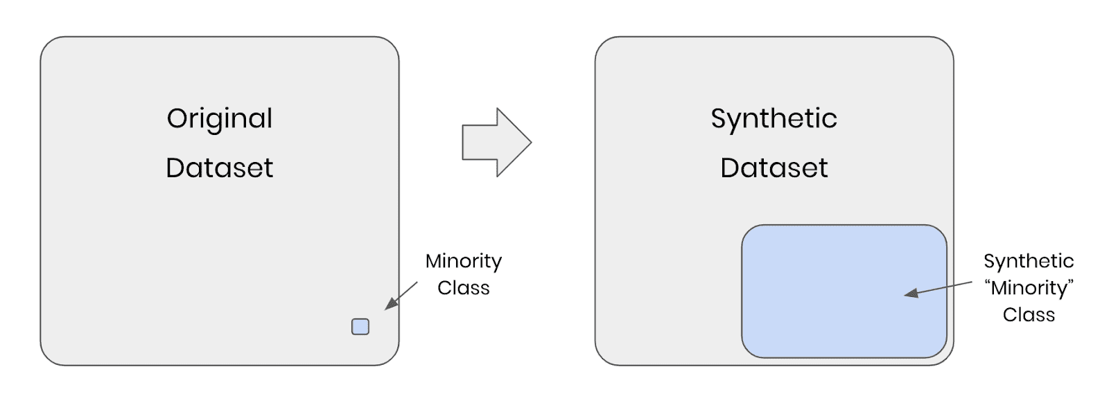
Fig 1 - Synthetic rebalancing creates more statistically representative instances of the minority class
Why should I rebalance my dataset?
In heavily imbalanced classification projects, a machine learning model has very little data to effectively learn patterns about the minority class. This will affect its ability to correctly class instances of this minority class in the real (non-training) data when the model is put into production. A common real-world example is credit card fraud detection: the overwhelming majority of credit card transactions are perfectly legitimate, but it is precisely the rare occurrences of illegitimate use that we would be interested in capturing.
Let’s say we have a training dataset with 100,000 credit card transactions which contains 999,900 legitimate transactions and 100 fraudulent ones. A machine-learning model trained on this dataset would have ample opportunity to learn about all the different kinds of legitimate transactions, but only a small sample of 100 records in which to learn everything it can about fraudulent behavior. Once this model is put into production, the probability is high that fraudulent transactions will occur that do not follow any of the patterns seen in the small training sample of 100 fraudulent records. The machine learning model is unlikely to classify these fraudulent transactions.
So how can we address this problem? We need to give our machine learning model more examples of fraudulent transactions in order to ensure optimal predictive performance in production. This can be achieved through rebalancing.
Rebalancing Methods
We will explore three types of rebalancing:
- Random (or “naive”) oversampling
- SMOTE upsampling
- Synthetic rebalancing
The tutorial will give you hands-on experience with each type of rebalancing and provide you with in-depth understanding of the differences between them so you can choose the right method for your use case. We’ll start by generating an imbalanced dataset and showing you how to perform synthetic rebalancing using MOSTLY AI's synthetic data generator. We will then compare performance metrics of each rebalancing method on a downstream ML task.
But first things first: we need some data.
Generate an Imbalanced Dataset
For this tutorial, we will be using the UCI Adult Income dataset, as well as the same training and validation split, that was used in the Train-Synthetic-Test-Real tutorial. However, for this tutorial we will work with an artificially imbalanced version of the dataset containing only 0.1% of high-income (>50K) records in the training data, by downsampling the minority class. The downsampling has already been done for you, but if you want to reproduce it yourself you can use the code block below:
def create_imbalance(df, target, ratio):
    val_min, val_maj = df[target].value_counts().sort_values().index
    df_maj = df.loc[df[target]==val_maj]
    n_min = int(df_maj.shape[0]/(1-ratio)*ratio)
    df_min = df.loc[df[target]==val_min].sample(n=n_min, random_state=1)
    df_maj = df.loc[df[target]==val_maj]
    df_imb = pd.concat([df_min, df_maj]).sample(frac=1, random_state=1)
    return df_imb

df_trn = pd.read_csv(f'{repo}/census-training.csv')
df_trn_imb = create_imbalance(df_trn, 'income', 1/1000)
df_trn_imb.to_csv('census-training-imbalanced.csv', index=False)
Let’s take a quick look at this imbalanced dataset by randomly sampling 10 rows. For legibility let’s select only a few columns, including the income column as our imbalanced feature of interest:
trn = pd.read_csv(f'{repo}/census-training-imbalanced.csv')
trn.sample(n=10)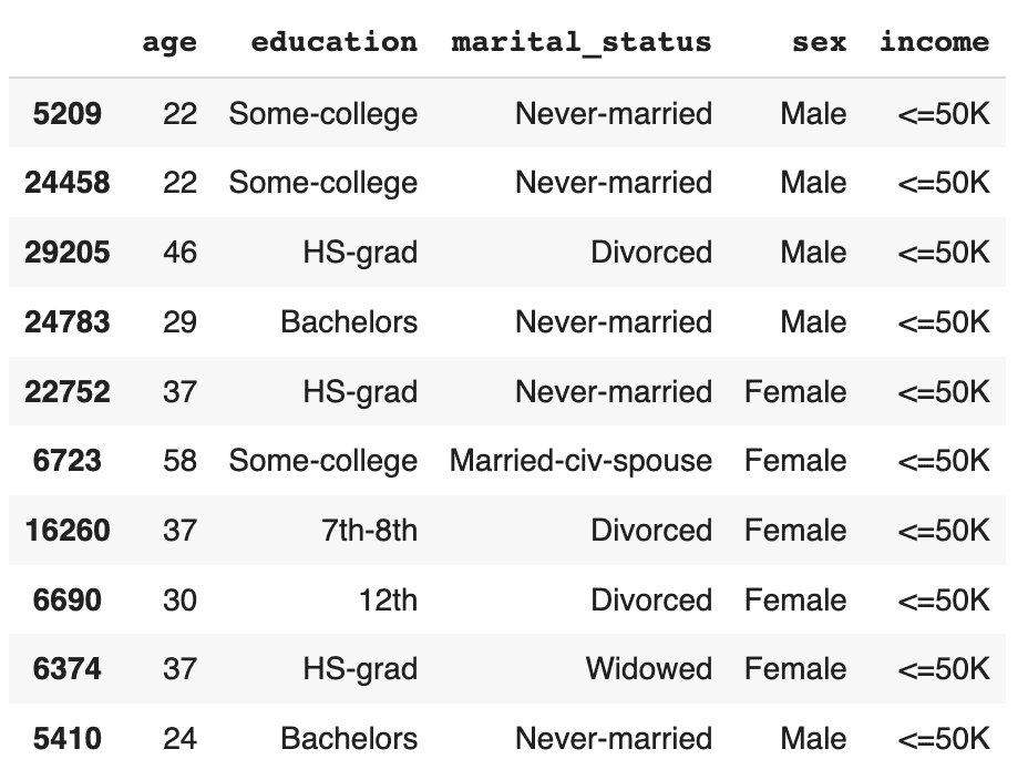
You can try executing the line above multiple times to see different samples. Still, due to the strong class imbalance, the chance of finding a record with high income in a random sample of 10 is minimal. This would be problematic if you were interested in creating a machine learning model that could accurately classify high-income records (which is precisely what we’ll be doing in just a few minutes).
The problem becomes even more clear when we try to sample a specific sub-group in the population. Let’s sample all the female doctorates with a high income in the dataset. Remember, the dataset contains almost 30 thousand records.
trn[
    (trn['income']=='>50K')
    & (trn.sex=='Female')
    & (trn.education=='Doctorate')
]
It turns out there are actually no records of this type in the training data. Of course, we know that these kinds of individuals exist in the real world and so our machine learning model is likely to encounter them when put in production. But having had no instances of this record type in the training data, it is likely that the ML model will fail to classify this kind of record correctly. We need to provide the ML model with a higher quantity and more varied range of training samples of the minority class to remedy this problem.
Synthetic rebalancing with MOSTLY AI
MOSTLY AI offers a synthetic rebalancing feature that can be used with any categorical column. Let’s walk through how this works:
- Download the imbalanced dataset here if you haven’t generated it yourself already. Use Ctrl+S or Cmd+S to save the file locally.
- Go to your MOSTLY AI account and navigate to “Synthetic Datasets”. Upload
census-training-imbalanced.csvand click “Proceed”.
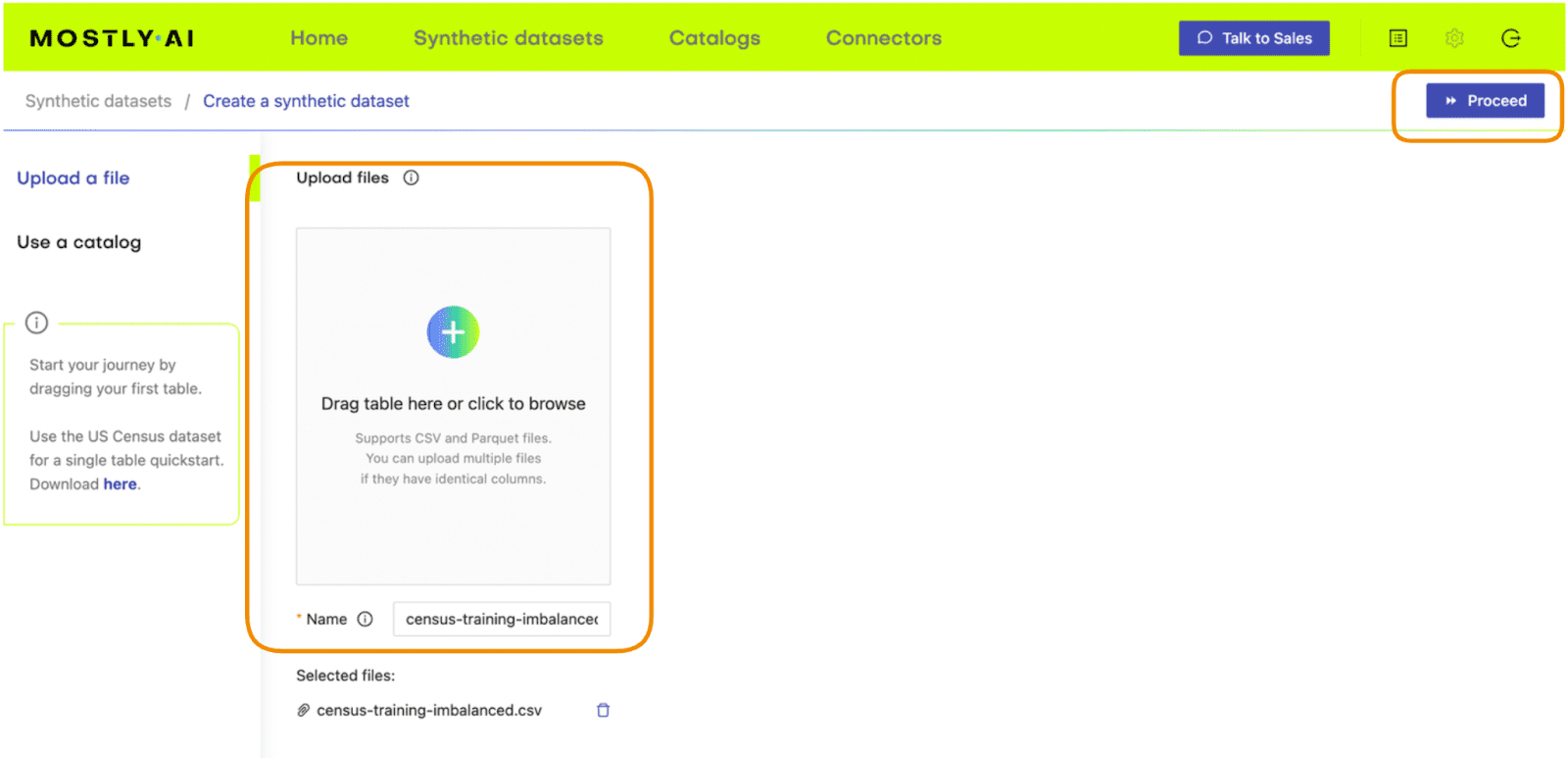
Fig 2 - Upload the original dataset to MOSTLY AI’s synthetic data generator.
- On the next page, click “Data Settings” and then click on the “Income” column
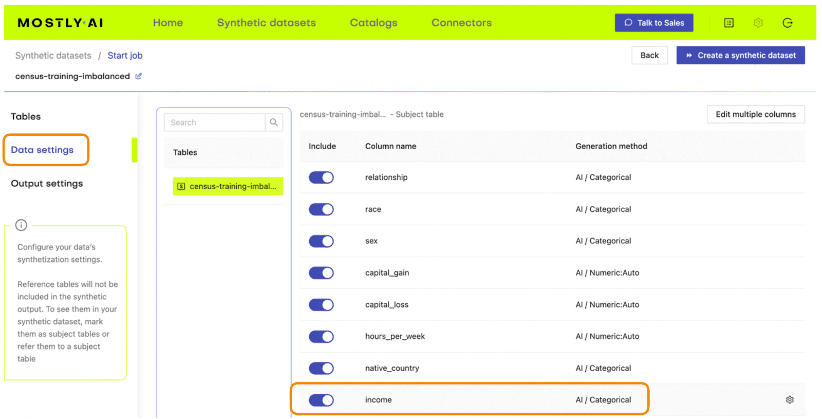
Fig 3 - Navigate to the Data Settings of the Income column.
- Set the Encoding Type to “Categorical” and select the option to “Use this column to rebalance the table”. Then add a new row and rebalance the “>50K” column to be “50%” of the dataset. This will synthetically upsample the minority class to create an even split between high-income and low-income records.
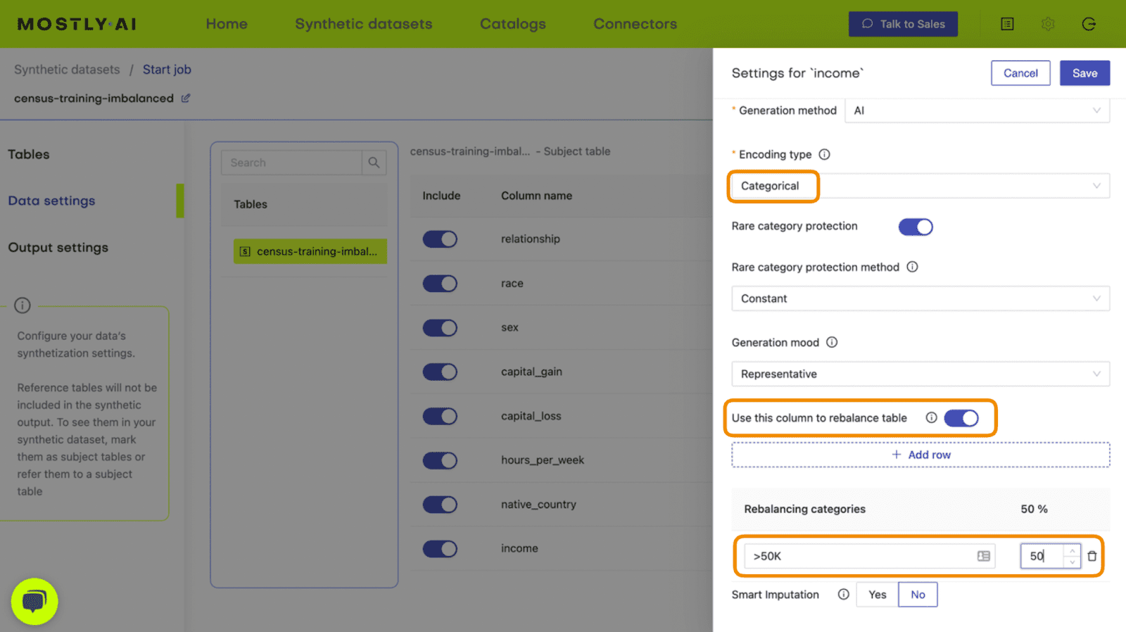
Fig 4 - Set the relevant settings to rebalance the income column.
- Click “Save” and on the next page click “Create a synthetic dataset” to launch the job.
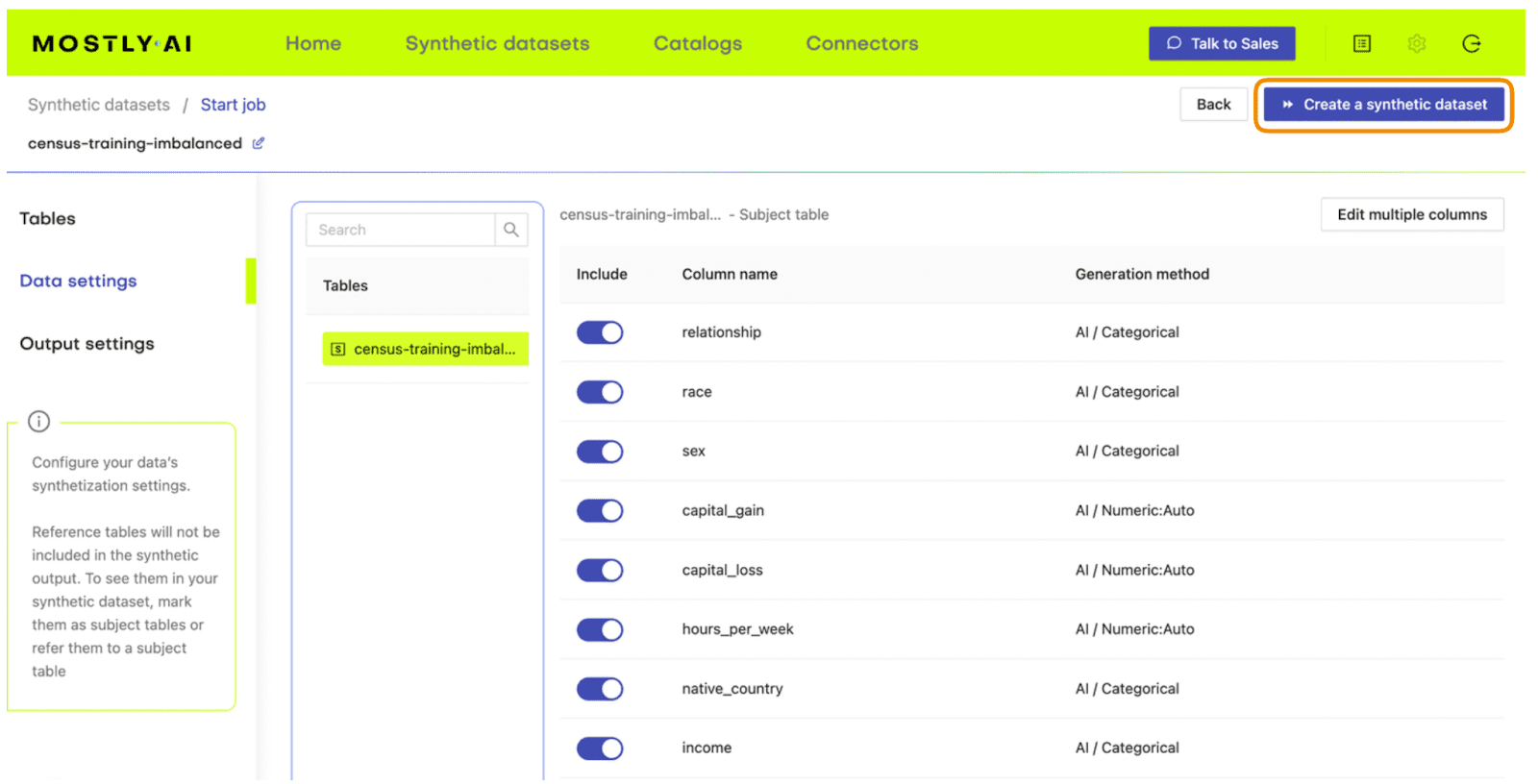
Fig 5 - Launch the synthetic data generation
Once the synthesization is complete, you can download the synthetic dataset to disk. Then return to wherever you are running your code and use the following code block to create a DataFrame containing the synthetic data.
# upload synthetic dataset
import pandas as pd

try:
    # check whether we are in Google colab
    from google.colab import files
    print("running in COLAB mode")
    repo = 'https://github.com/mostly-ai/mostly-tutorials/raw/dev/rebalancing'
    import io
    uploaded = files.upload()
    syn = pd.read_csv(io.BytesIO(list(uploaded.values())[0]))
    print(f"uploaded synthetic data with {syn.shape[0]:,} records and {syn.shape[1]:,} attributes")
except:
    print("running in LOCAL mode")
    repo = '.'
    print("adapt `syn_file_path` to point to your generated synthetic data file")
    syn_file_path = './census-synthetic-balanced.csv'
    syn = pd.read_csv(syn_file_path)
    print(f"read synthetic data with {syn.shape[0]:,} records and {syn.shape[1]:,} attributes")
Let's now repeat the data exploration steps we performed above with the original, imbalanced dataset. First, let’s display 10 randomly sampled synthetic records. We'll subset again for legibility. You can run this line multiple times to get different samples.
# sample 10 random records
syn_sub = syn[['age','education','marital_status','sex','income']]
syn_sub.sample(n=10)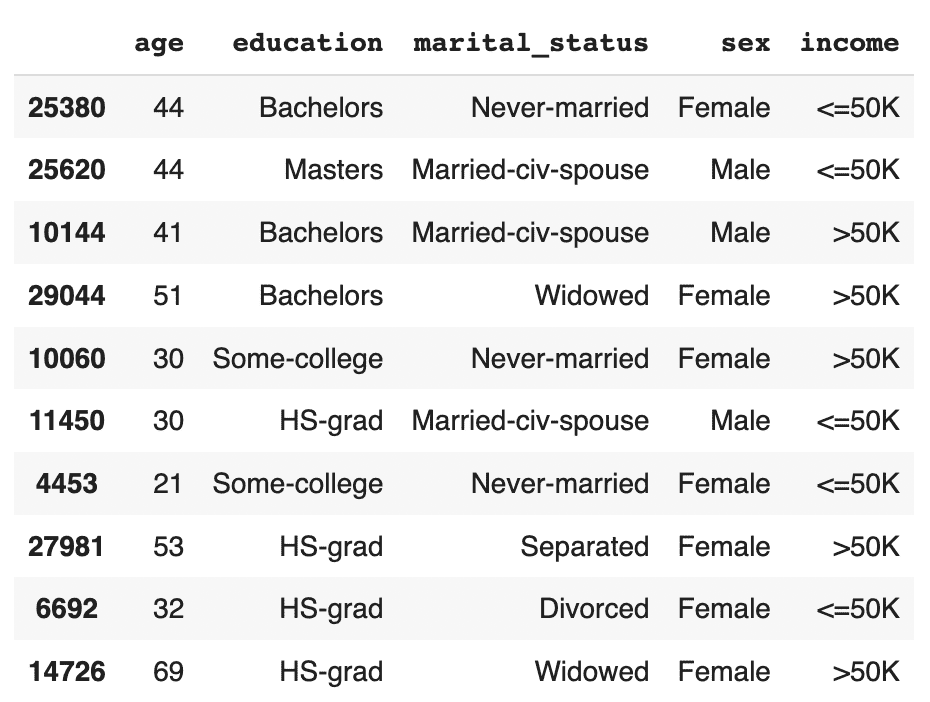
This time, you should see that the records are evenly distributed across the two income classes.
Let's now investigate all female doctorates with a high income in the synthetic, rebalanced dataset:
syn_sub[
    (syn_sub['income']=='>50K')
    & (syn_sub.sex=='Female')
    & (syn_sub.education=='Doctorate')
].sample(n=10)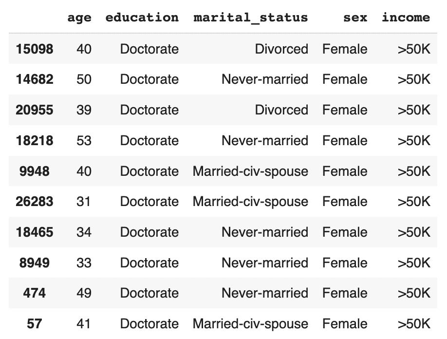
The synthetic data contains a list of realistic, statistically sound female doctorates with a high income. This is great news for our machine learning use case because it means that our ML model will have plenty of data to learn about this particular important subsegment.
Evaluate ML performance using TSTR
Let’s now compare the quality of different rebalancing methods by training a machine learning model on the rebalanced data and evaluating the predictive performance of the resulting models.
We will investigate and compare 3 types of rebalancing:
- Random (or “naive”) oversampling
- SMOTE upsampling
- Synthetic rebalancing
The code block below defines the functions that will preprocess your data, train a LightGBM model and evaluate its performance using a holdout dataset. For more detailed descriptions of this code, take a look at the Train-Synthetic-Test-Real tutorial.
# import necessary libraries
import lightgbm as lgb
from lightgbm import early_stopping
from sklearn.model_selection import train_test_split
from sklearn.metrics import roc_auc_score, f1_score
import seaborn as sns
import matplotlib.pyplot as plt

# define target column and value
target_col = 'income'
target_val = '>50K'

# define preprocessing function
def prepare_xy(df: pd.DataFrame):
    y = (df[target_col]==target_val).astype(int)
    str_cols = [
        col for col in df.select_dtypes(['object', 'string']).columns if col != target_col
    ]
    for col in str_cols:
        df[col] = pd.Categorical(df[col])
    cat_cols = [
        col for col in df.select_dtypes('category').columns if col != target_col
    ]
    num_cols = [
        col for col in df.select_dtypes('number').columns if col != target_col
    ]
    for col in num_cols:
        df[col] = df[col].astype('float')
    X = df[cat_cols + num_cols]
    return X, y

# define training function
def train_model(X, y):
    cat_cols = list(X.select_dtypes('category').columns)
    X_trn, X_val, y_trn, y_val = train_test_split(X, y, test_size=0.2, random_state=1)
    ds_trn = lgb.Dataset(
        X_trn,
        label=y_trn,
        categorical_feature=cat_cols,
        free_raw_data=False
    )
    ds_val = lgb.Dataset(
        X_val,
        label=y_val,
        categorical_feature=cat_cols,
        free_raw_data=False
    )
    model = lgb.train(
        params={
            'verbose': -1,
            'metric': 'auc',
            'objective': 'binary'
         },
         train_set=ds_trn,
         valid_sets=[ds_val],
         callbacks=[early_stopping(5)],
    )
    return model

# define evaluation function
def evaluate_model(model, hol):
    X_hol, y_hol = prepare_xy(hol)
    probs = model.predict(X_hol)
    preds = (probs >= 0.5).astype(int)
    auc = roc_auc_score(y_hol, probs)
    f1 = f1_score(y_hol, probs>0.5, average='macro')
    probs_df = pd.concat([
        pd.Series(probs, name='probability').reset_index(drop=True),
        pd.Series(y_hol, name=target_col).reset_index(drop=True)
    ], axis=1)
    sns.displot(
        data=probs_df,
        x='probability',
        hue=target_col,
        bins=20,
        multiple="stack"
     )
    plt.title(f"AUC: {auc:.1%}, F1 Score: {f1:.2f}", fontsize = 20)
    plt.show()
    return auc

# create holdout dataset
df_hol = pd.read_csv(f'{repo}/census-holdout.csv')
df_hol_min = df_hol.loc[df_hol['income']=='>50K']
print(f"Holdout data consists of {df_hol.shape[0]:,} records",
f"with {df_hol_min.shape[0]:,} samples from the minority class")
ML performance of imbalanced dataset
Let’s now train a LightGBM model on the original, heavily imbalanced dataset and evaluate its predictive performance. This will give us a baseline against which we can compare the performance of the different rebalanced datasets.
X_trn, y_trn = prepare_xy(trn)
model_trn = train_model(X_trn, y_trn)
auc_trn = evaluate_model(model_trn, df_hol)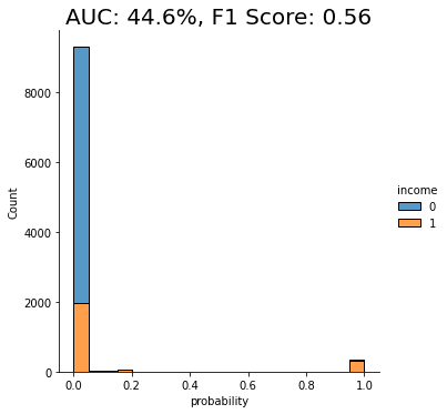
With an AUC of about 50%, the model trained on the imbalanced dataset is just as good as a flip of a coin, or, in other words, not worth very much at all. The downstream LightGBM model is not able to learn any signal due to the low number of minority-class samples.
Let’s see if we can improve this using rebalancing.
Naive rebalancing
First, let’s rebalance the dataset using the random oversampling method, also known as “naive rebalancing”. This method simply takes the minority class records and copies them to increase their quantity. This increases the number of records of the minority class but does not increase the statistical diversity. We will use the imblearn library to perform this step, feel free to check out their documentation for more context.
The code block performs the naive rebalancing, trains a LightGBM model using the rebalanced dataset and evaluates its predictive performance:
from imblearn.over_sampling import RandomOverSampler

X_trn, y_trn = prepare_xy(trn)
sm = RandomOverSampler(random_state=1)
X_trn_up, y_trn_up = sm.fit_resample(X_trn, y_trn)
model_trn_up = train_model(X_trn_up, y_trn_up)
auc_trn_up = evaluate_model(model_trn_up, df_hol)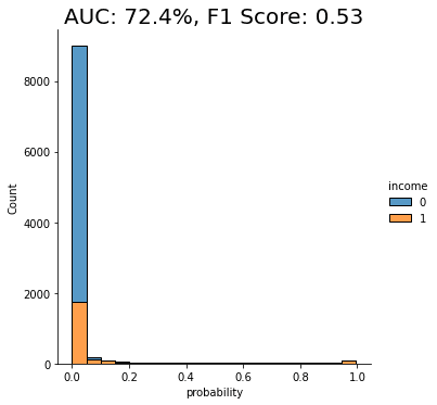
We see a clear improvement in predictive performance, with an AUC score of around 70%. This is better than the baseline model trained on the imbalanced dataset, but still not great. We see that a significant portion of the “0” class (low-income) is being incorrectly classified as “1” (high-income).
This is not surprising because, as stated above, this rebalancing method just copies the existing minority class records. This increases their quantity but does not add any new statistical information into the model and therefore does not offer the model much data that it can use to learn about minority-class instances that are not present in the training data.
Let’s see if we can improve on this using another rebalancing method.
SMOTE rebalancing
SMOTE upsampling is a state-of-the art upsampling method which, unlike the random oversampling seen above, does create novel, statistically representative samples. It does so by interpolating between neighboring samples. It’s important to note, however, that SMOTE upsampling is non-privacy-preserving.
The following code block performs the rebalancing using SMOTE upsampling, trains a LightGBM model on the rebalanced dataset, and evaluates its performance:
from imblearn.over_sampling import SMOTENC

X_trn, y_trn = prepare_xy(trn)
sm = SMOTENC(
    categorical_features=X_trn.dtypes=='category',
    random_state=1
)
X_trn_smote, y_trn_smote = sm.fit_resample(X_trn, y_trn)
model_trn_smote = train_model(X_trn_smote, y_trn_smote)
auc_trn_smote = evaluate_model(model_trn_smote, df_hol)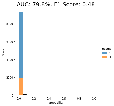
We see another clear jump in performance: the SMOTE upsampling boosts the performance of the downstream model to close to 80%. This is clearly an improvement from the random oversampling we saw above, and for this reason, SMOTE is quite commonly used.
Let’s see if we can do even better.
Synthetic rebalancing with MOSTLY AI
In this final step, let’s take the synthetically rebalanced dataset that we generated earlier using MOSTLY AI to train a LightGBM model. We’ll then evaluate the performance of this downstream ML model and compare it against those we saw above.
The code block below prepares the synthetically rebalanced data, trains the LightGBM model, and evaluates it:
X_syn, y_syn = prepare_xy(syn)
model_syn = train_model(X_syn, y_syn)
auc_syn = evaluate_model(model_syn, df_hol)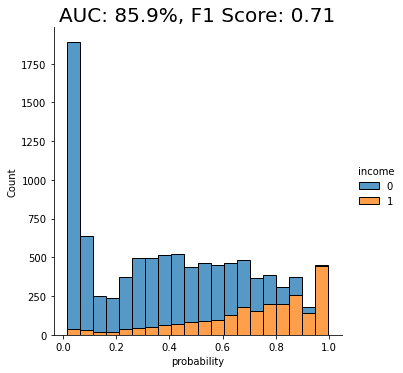
Both performance measures, the AUC as well as the macro-averaged F1 score, are significantly better for the model that was trained on synthetic data than if it were trained on any of the other methods. We can also see that the portion of “0”s incorrectly classified as “1”s has dropped significantly.
The synthetically rebalanced dataset has enabled the model to make fine-grained distinctions between the high-income and low-income records. This is strong proof of the value of synthetic rebalancing for learning more about a small sub-group within the population.
The value of synthetic rebalancing
In this tutorial, you have seen firsthand the value of synthetic rebalancing for downstream ML classification problems. You have gained an understanding of the necessity of rebalancing when working with imbalanced datasets in order to provide the machine learning model with more samples of the minority class. You have learned how to perform synthetic rebalancing with MOSTLY AI and observed the superior performance of this rebalancing method when compared against other methods on the same dataset. Of course, the actual lift in performance may vary depending on the dataset, the predictive task, and the chosen ML model.
What’s next?
In addition to walking through the above instructions, we suggest experimenting with the following in order to get an even better grasp of synthetic rebalancing:
- repeat the experiments for different class imbalances,
- repeat the experiments for different datasets, ML models, and predictive tasks.