In this tutorial, you will explore the relationship between the size of your training sample and synthetic data accuracy. This is an important concept to master because it can help you significantly reduce the runtime and computational cost of your training runs while maintaining the optimal accuracy you require.

We will start with a single real dataset, which we will use to create 5 different synthetic datasets, each with a different training sample size. We will then evaluate the accuracy of the 5 resulting synthetic datasets by looking at individual variable distributions, by verifying rule-adherence and by evaluating their performance on a downstream machine-learning (ML) task. The Python code for this tutorial is runnable and publicly available in this Google Colab notebook.

Size vs synthetic data accuracy tradeoff

Our working hypothesis is that synthetic data accuracy will increase as the number of training samples increases: the more data the generative AI model has to learn from, the better it will perform. 

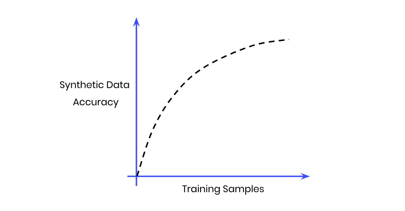
Fig 1 - The Size vs Accuracy Tradeoff

But more training samples also means more data to crunch; i.e. more computational cost and a longer runtime. Our goal, then, will be to find the sweet spot at which we achieve optimal accuracy with the lowest number of training samples possible. 

Note that we do not expect synthetic data to ever perfectly match the original data. This would only be satisfied by a copy of the data, which obviously would neither satisfy any privacy requirements nor would provide any novel samples. That being said, we shall expect that due to sampling variance the synthetic data can deviate. Ideally this deviation will be just as much, and not more, than the deviation that we would observe by analyzing an actual holdout dataset.

Synthesize your data

For this tutorial, we will be using the same UCI Adult Income dataset, as well as the same training and validation split, that was used in the Train-Synthetic-Test-Real tutorial. This means we have a total of 48,842 records across 15 attributes, and will be using up to 39,074 (=80%) of those records for the synthesis.

1. Download the training data census-training.csv by clicking here and pressing Ctrl+S or Cmd+S to save the file locally. This is an 80% sample of the full dataset. The remaining 20% sample (which we’ll use for evaluation later) can be fetched from here.

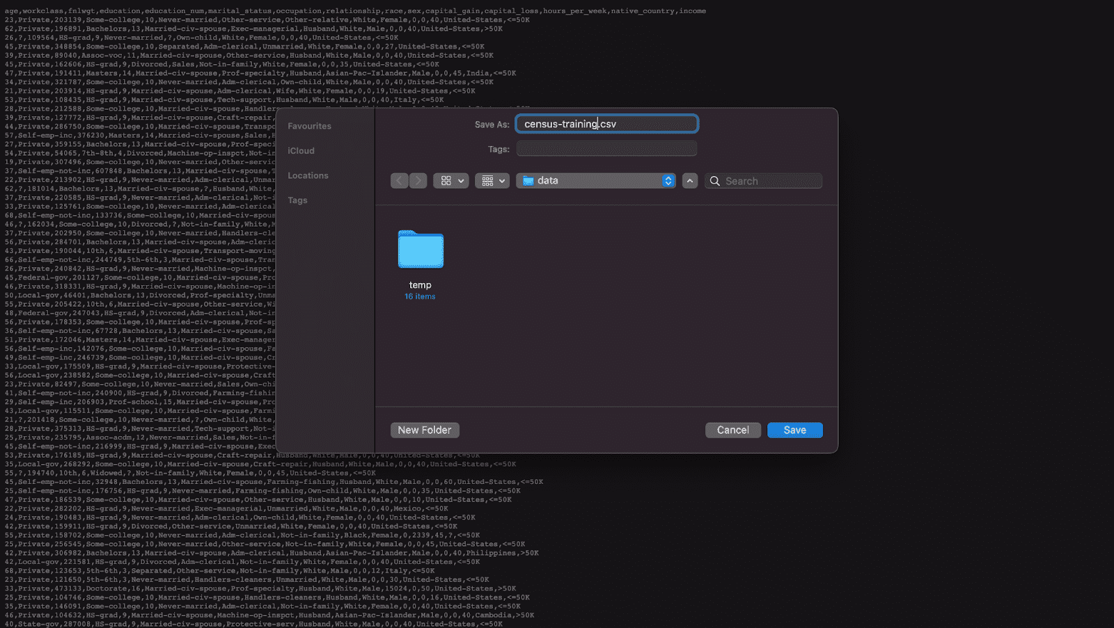
Fig 2 - Download the original training data and save it to disk.

2. Synthesize census-training.csv via MOSTLY AI's synthetic data generator multiple times, each time with a different number of maximum training samples. We will use the following training sample sizes in this tutorial: 100, 400, 1600, 6400, 25600. Always generate a consistent number of subjects, e.g. 10,000. You can leave all other settings at their default.
   
3. Download the generated datasets from MOSTLY AI as CSV files, and rename each CSV file with an appropriate name (eg. syn_00100.csv, syn_00400.csv, etc.)

4. Now ensure you can access the synthetic datasets from wherever you are running the code for this tutorial. If you are working from the Colab notebook, you can upload the synthetic datasets by executing the code block below:

# upload synthetic dataset
import pandas as pd
try:
    # check whether we are in Google colab
    from google.colab import files
    print("running in COLAB mode")
    repo = 'https://github.com/mostly-ai/mostly-tutorials/raw/dev/size-vs-accuracy'
    import io
    uploaded = files.upload()
    synthetic_datasets = {
        file_name: pd.read_csv(io.BytesIO(uploaded[file_name]), skipinitialspace=True)
        for file_name in uploaded
    }
except:
    print("running in LOCAL mode")
    repo = '.'
    print("upload your synthetic data files to this directory via Jupyter")
    from pathlib import Path
    syn_files = sorted(list(Path('.').glob('syn*csv')))
    synthetic_datasets = {
        file_name.name: pd.read_csv(file_name)
        for file_name in syn_files
    }


for k, df in synthetic_datasets.items():
    print(f"Loaded Dataset `{k}` with {df.shape[0]:,} records and {df.shape[1]:,} attributes")

Evaluate synthetic data accuracy

Now that you have your 5 synthetic datasets (each trained on a different training sample size) let’s take a look at the high-level accuracy scores of these synthetic datasets.

1. Navigate to your MOSTLY AI account and note the reported overall synthetic data accuracy as well as the runtime of each job:

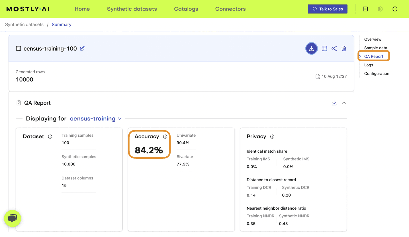
Fig 3 - Note the accuracy score in the QA Report tab of your completed synthetic dataset job.

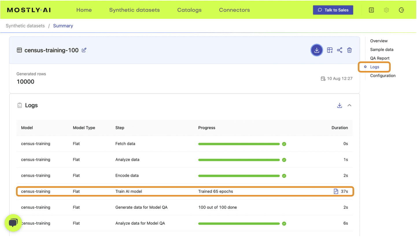
Fig 4 - Note the training time from the Logs tab.

2. Update the following DataFrame accordingly:

results = pd.DataFrame([
{'file': 'syn_00100.csv', 'samples': 100, 'accuracy': 0.830, 'runtime': 37},
{'file': 'syn_00400.csv', 'samples': 400, 'accuracy': 0.914, 'runtime': 45},
{'file': 'syn_01600.csv', 'samples': 1600, 'accuracy': 0.956, 'runtime': 48},
{'file': 'syn_06400.csv', 'samples': 6400, 'accuracy': 0.972, 'runtime': 54},
{'file': 'syn_25600.csv', 'samples': 25600, 'accuracy': 0.980, 'runtime': 75},
])
results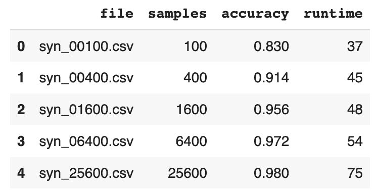

3. Visualize the results using the code block below:

import seaborn as sns
import matplotlib.pyplot as plt

sns.catplot(data=results, y='accuracy', x='file', kind='point', color='black')
plt.xticks(rotation=45)
plt.xlabel('')
plt.title('QA Report - Overall Accuracy')
plt.show()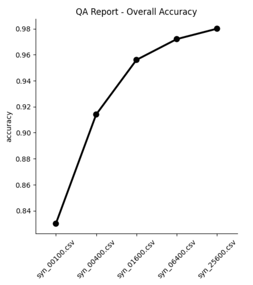

From both the table and the plot we can see that, as expected, the overall accuracy of the synthetic data improves as we increase the number of training samples. But notice that the increase is not strictly linear: while we see big jumps in accuracy performance between the first three datasets (100, 400 and 1,600 samples, respectively), the jumps get smaller as the training samples increase in size. Between the last two datasets (trained on 6,400 and 25,600 samples, respectively) the increase in accuracy is less than 0.1%, while the runtime increases by more than 35%.

Synthetic data quality deep-dive

The overall accuracy score is a great place to start when assessing the quality of your synthetic data, but let’s now dig a little deeper to see how the synthetic dataset compares to the original data from a few different angles. We’ll take a look at:

• Distributions of individual variables
• Rule adherence
• Performance on a downstream ML task 

Before you jump into the next sections, run the code block below to concatenate all the 5 synthetic datasets together in order to facilitate comparison:

# combine synthetics
df = pd.concat([d.assign(split=k) for k, d in synthetic_datasets.items()], axis=0)
df['split'] = pd.Categorical(df['split'], categories=df["split"].unique())
df.insert(0, 'split', df.pop('split'))

# combine synthetics and original
df_trn = pd.read_csv(f'{repo}/census-training.csv')
df_hol = pd.read_csv(f'{repo}/census-holdout.csv')
dataset = synthetic_datasets | {'training': df_trn, 'holdout': df_hol}
df_all = pd.concat([d.assign(split=k) for k, d in dataset.items()], axis=0)
df_all['split'] = pd.Categorical(df_all['split'], categories=df_all["split"].unique())
df_all.insert(0, 'split', df_all.pop('split'))

Single variable distributions

Let’s explore the distributions of some individual variables.

The more training samples have been used for the synthesis, the closer the synthetic distributions are expected to be to the original ones. Note that we can also see deviations within statistics between the target and the holdout data. This is expected due to the sampling variance. The smaller the dataset, the larger the sampling variance will be. The ideal synthetic dataset would deviate from the original dataset just as much as the holdout set does.

Start by taking a look at the average age, split by marital status:

stats = (
    df_all.groupby(['split', 'marital_status'])['age']
    .mean().round().to_frame().reset_index(drop=False)
)
stats = (
    stats.loc[~stats['marital_status']
    .isin(['_RARE_', 'Married-AF-spouse', 'Married-spouse-absent', 'Separated'])]
)
stats = (
    stats.pivot_table(index='split', columns=['marital_status'])
    .reset_index(drop=False)
)
stats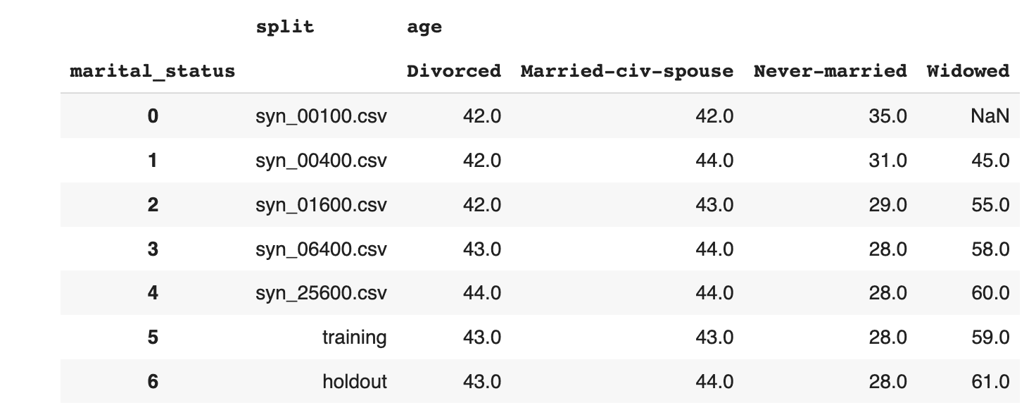

Then explore the age distribution, split by income:

sns.catplot(
    data=df_all, 
    x='age', 
    y='split', 
    hue='income', 
    kind='violin', 
    split=True, 
    legend=None
)
plt.legend(loc='upper right', title='', prop={'size': 8})
plt.show()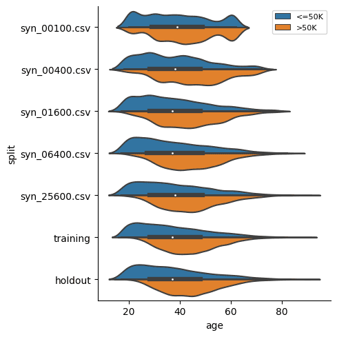

In both of these cases we see, again, that the synthetic datasets trained on more training samples resemble the original dataset more closely. We also see that the difference between the dataset trained on 6,400 samples and that trained on 25,600 seems to be minimal. This means that if the accuracy of these specific individual variable distributions is most important to you, you could confidently train your synthetic data generation model using just 6,400 samples (rather than the full 39,074 records). This will save you significantly in computational costs and runtime.

Rule Adherence

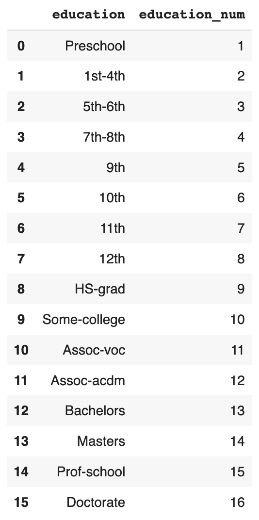
The original data has a 1:1 relationship between the education and education_num columns: each textual education level in the education column has a corresponding numerical value in the education_num column.

Let's check in how many cases the generated synthetic data has correctly retained that specific rule between these two columns.

First, display the matching columns in the original training data:

# display unique combinations of `education` and `education_num`
(df_trn[['education', 'education_num']]
 .drop_duplicates()
 .sort_values('education_num')
 .reset_index(drop=True)
)

Now, convert the education column to Categorical dtype, sort and calculate the ratio of correct matches:

# convert `education` to Categorical with proper sort order
df['education'] = pd.Categorical(
    df['education'], 
    categories=df_trn.sort_values('education_num')['education'].unique())

# calculate correct match
stats = (
    df.groupby('split')
    .apply(lambda x: (x['education'].cat.codes+1 == x['education_num']).mean())
)
stats = stats.to_frame('matches').reset_index()
stats

Visualize the results:

sns.catplot(
    data=stats, 
    y='matches', 
    x='split', 
    kind='point', 
    color='black'
)
plt.xticks(rotation=45)
plt.xlabel('')
plt.title('Share of Matches')
plt.show()

We can see from both the table and the plot that the dataset trained on just 100 samples severely underperforms, matching the right values in the columns only half of the time. While performance improves as the training samples increase, only the synthetic dataset generated using 25,600 samples is able to reproduce this rule adherence 100%. This means that if rule adherence for these columns is crucial to the quality of your synthetic data, you should probably opt for a training size of 25,600.

Downstream ML task

Finally, let’s evaluate the 5 synthetic datasets by evaluating their performance on a downstream machine learning task. This is also referred to as the Train-Synthetic-Test-Real evaluation methodology. You will train a ML model on each of the 5 synthetic datasets and then evaluate them on their performance against an actual holdout dataset containing real data which the ML model has never seen before (the remaining 20% of the dataset, which can be downloaded here).

The code block below defines the functions that will preprocess your data, train a LightGBM model and evaluate its performance. For more detailed descriptions of this code, take a look at the Train-Synthetic-Test-Real tutorial.

# import necessary libraries
import lightgbm as lgb
from lightgbm import early_stopping
from sklearn.model_selection import train_test_split
from sklearn.metrics import roc_auc_score

# define target column and value
target_col = 'income'
target_val = '>50K'

# prepare data, and split into features `X` and target `y`
def prepare_xy(df: pd.DataFrame):
    y = (df[target_col]==target_val).astype(int)
    str_cols = [
        col for col in df.select_dtypes(['object', 'string']).columns if col != target_col
    ]
    for col in str_cols:
        df[col] = pd.Categorical(df[col])
    cat_cols = [
        col for col in df.select_dtypes('category').columns if col != target_col
    ]
    num_cols = [
        col for col in df.select_dtypes('number').columns if col != target_col
    ]
    for col in num_cols:
        df[col] = df[col].astype('float')
    X = df[cat_cols + num_cols]
    return X, y


# train ML model with early stopping
def train_model(X, y):
    cat_cols = list(X.select_dtypes('category').columns)
    X_trn, X_val, y_trn, y_val = train_test_split(X, y, test_size=0.2, random_state=1)
    ds_trn = lgb.Dataset(
        X_trn, 
        label=y_trn, 
        categorical_feature=cat_cols, 
        free_raw_data=False
    )
    ds_val = lgb.Dataset(
        X_val, 
        label=y_val, 
        categorical_feature=cat_cols, 
        free_raw_data=False
    )
    model = lgb.train(
        params={
            'verbose': -1,
            'metric': 'auc',
            'objective': 'binary'
        },
        train_set=ds_trn,
        valid_sets=[ds_val],
        callbacks=[early_stopping(5)],
    )
    return model


# apply ML Model to some holdout data, report key metrics, and visualize scores
def evaluate_model(model, hol):
    X_hol, y_hol = prepare_xy(hol)
    probs = model.predict(X_hol)
    preds = (probs >= 0.5).astype(int)
    auc = roc_auc_score(y_hol, probs)
    return auc


def train_and_evaluate(df):
    X, y = prepare_xy(df)
    model = train_model(X, y)
    auc = evaluate_model(model, df_hol)
    return auc

Now calculate the performance metric for each of the 5 ML models:

aucs = {k: train_and_evaluate(df) for k, df in synthetic_datasets.items()}
aucs = pd.Series(aucs).round(3).to_frame('auc').reset_index()

And visualize the results:

sns.catplot(
    data=aucs, 
    y='auc', 
    x='index', 
    kind='point', 
    color='black'
)
plt.xticks(rotation=45)
plt.xlabel('')
plt.title('Predictive Performance (AUC) on Holdout')
plt.show()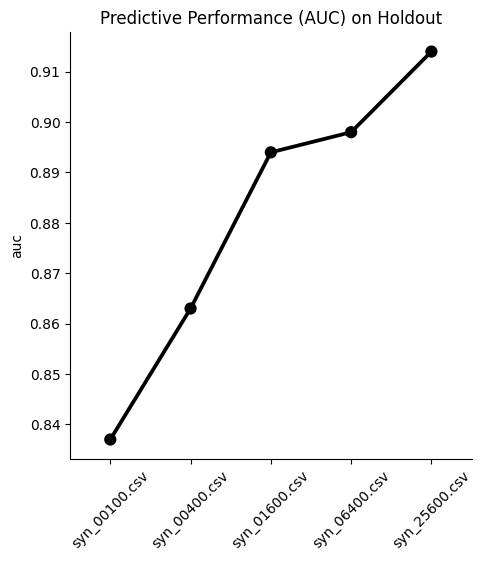

We see, again, that optimal performance is achieved with the largest training sample size. Interestingly, the difference in performance between the dataset trained on 1,600 samples and the one trained on 6,400 samples is minimal in this case. This means that if your use case allows you to sacrifice a fraction of ML performance, you could train your synthetic data generator on just 1,600 samples and still get pretty great results.

In most cases, however, a 1% difference in ML accuracy is crucial to preserve and so most likely you would end up training on 25,600 samples. A worthwhile exercise here would be to train a synthetic generator using the full 39,074 training samples to see whether that performs even better.

Optimize your training sample size for synthetic data accuracy

In this tutorial you have seen first-hand the relationship between the size of your training samples and the resulting synthetic data quality. You have quantified and evaluated this relationship from multiple angles and with various use cases in mind, including looking at single variable distributions, rule adherence and ML utility. For the given dataset and the given synthesizer we can clearly observe an increase in synthetic data quality with a growing number of training samples across the board.  

We have also observed that a holdout dataset will exhibit deviations from the training data due to sampling variance. With the holdout data being actual data that hasn't been seen before, it serves as a north star in terms of maximum achievable synthetic data accuracy. Read our blog post on benchmarking synthetic data generators for more on this topic.

What’s next?

In addition to walking through the above instructions, we suggest experimenting with the following in order to get an even better grasp of the relationship between training sample size and synthetic data accuracy:

• to limit model training to a few epochs, e.g. by setting the maximum number of epochs to 1 or 5 and study its impact on runtime and quality.
• to synthesize with different model_sizes: Small, Medium and Large, and study its impact on runtime and quality.
• to synthesize with the same settings several times to study the variability in quality across several runs.
• to calculate and compare your own statistics, and then compare the deviations between synthetic and training. The deviations between holdout and training can serve as a benchmark.